Discriminative Active Learning
If you made it this far, you’ve been introduced to the active learning framework, saw how to extend the framework to more realistic settings and have seen ways of comparing active learning methods. We’ll now detail the thought process and experiments we ran when trying to come up with a new method - Discriminative Active Learning (DAL).
Intuition
We started with a simple idea - when we are creating a dataset to be labeled that we want to represent the original distribution well, we shouldn’t have too many redundant instances. If we want to learn from new examples, we want them to be different from what we already have.
So, if we were able to look at the unlabeled dataset and find the examples which are the most different from those in our labeled dataset, then picking them will hopefully give us informative samples to learn from.
The Method
If you buy into this intuition, it isn’t hard to think of a method that does just what we want:
Given a labeled set and an unlabeled set that we want to sample a batch from, instead of training a model to solve the original task on the labeled set, we train a model to classify between the labeled set and the unlabeled set. We then use that model to choose the examples which are most confidently classified as being from the unlabeled set.
Note that the label distribution here is very different from a regular binary classification task - two identical instances of the original distribution can be labeled differently simply depending on whether they’ve been labeled. This classification task resembles classifying a random labeling more than it does anything else…
Assuming our model can’t classify random labels perfectly with 0 loss, we should expect it to more confidently classify unlabeled examples which are far on the data manifold from labeled examples. This behavior should resemble the core set behavior, without being batch aware. Note that if the classifier is expressive enough to completely overfit the data and get a loss of 0, we can just stop training it before that happens.
The Representation
There are three possible representations we can use to train our binary classifier on:
The first is the raw data, which means we are completely agnostic to the labels and the task and can run our algorithm asynchronously from the labeling process (which is very nice). That said, this representation makes it hard for the binary classifier to pick up on semantic differences in the data, because it trains on a random labeling of the data. This representation has the advantage of decoupling the active learning process from the labeling process but will possibly give us poor results.
A second representation that decouples the active learning process from the labeling process is an autoencoder embedding of the data in a lower dimension. This representation has a higher chance of capturing some semantics about the data.
The final representation, like in the core set approach, is the representation learned by a model that is trained on the labeled data. This means our representation will contain more semantic features but will mean we are bound to the labeling process if we want to use a representation that improves throughout the active learning process.
Why This May Be Promising
This idea takes a very different approach to other active learning methods, in that it is completely agnostic about the original problem we are trying to solve, and only focuses on making the labeled set as diverse as possible. In this sense it is similar to the core set approach. This gives it the nice property that there is no need to adapt it to different machine learning scenarios like regression, segmentation, structured learning and so on.
Another bonus here, is that binary classification is relatively easy. It isn’t hard to overfit on two classes (even under random labels) with a modestly sized neural network, and it can be done rather quickly. The MIP formulation of the core set approach for instance is relatively slow and doesn’t scale as well.
Lastly, you may say that a conceptual drawback of our method is the fact that it isn’t batch-aware like the core set approach. The thing is, since we do not care about the actual labels of the data and only care about whether they are labeled or not, we can transfer chosen examples to the labeled set automatically without needing to wait for an annotator. This means we can trade off speed for batch awareness, by iteratively sampling sub-batches instead of the full batch. For example, if our batch size is 100, we can iteratively train the binary classifier, select 10 examples to be “labeled” and then retrain the binary classifier and keep going until we have our final batch of 100 examples.
Starting Out Small
So now that we’re motivated about our new algorithm, we can implement it on a toy problem and see how it compares to uncertainty sampling. We’ll use the MNIST dataset as our toy problem, trying to classify the digits “3” and “5” like we did in the introduction (with the representation being the raw data and a logistic regression model):
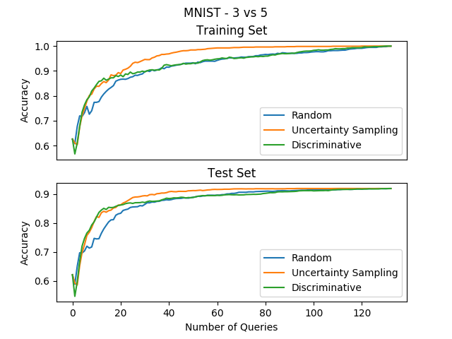
We can see that our method starts out really well, even beating uncertainty sampling a bit(!), but as the experiment progresses we see that it improves more and more slowly until it reaches accuracies that are the same as random sampling… This appears promising, but we must figure out what happens after the first few iterations that screws our method up.
Having this kind of unexpected behavior means we’re not understanding something basic about our method… So, let’s make things as simple as possible in order to understand what’s going on - let’s look at how our method behaves on synthetic 2-dimensional data. Like we did before, we’ll make two blobs that are linearly separable and look at what examples our method chooses:
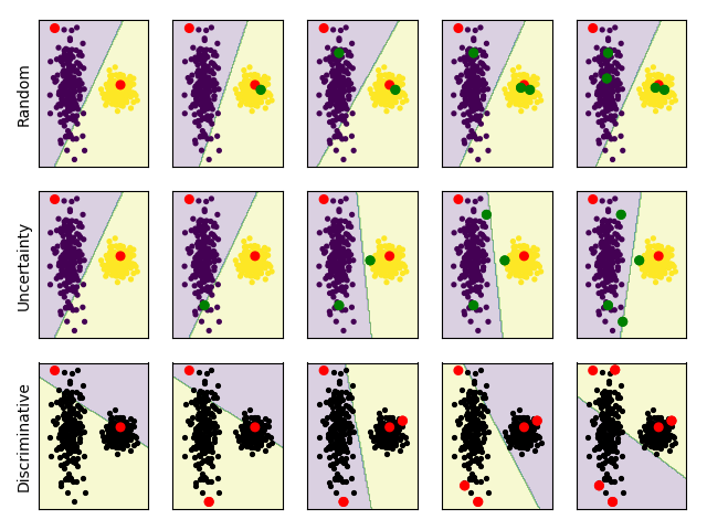
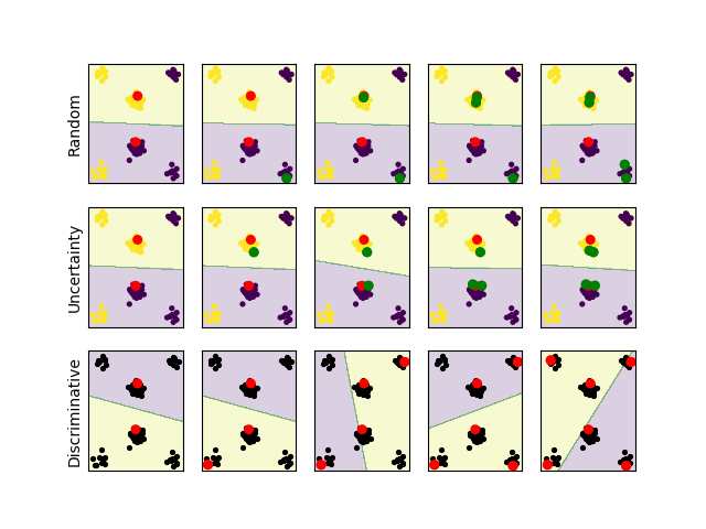
We color discriminative plots differently - red dots are in the labeled set and black dots are unlabeled. The decision boundary is also different, with the yellow part being areas classified as “unlabeled”. Before we analyze these results, let’s take a look at another synthetic blobby dataset and analyze them together:
This sort of data is very different from real data. We can’t really picture high dimensional data manifolds and our lower dimensional intuitions often fail in high dimensions. still, we can learn a thing or two from looking at toy problems. We can see that in the two cases our method is very different from uncertainty sampling:
In the first case, uncertainty sampling focuses heavily on examples which are close to the decision boundary between the two blobs, while our method does the opposite and focuses on examples in the extremes. In hindsight this isn’t very surprising - since our method chooses examples which are most confidently classified as “unlabeled”, when we’re working with linear classifiers like in this example our method chooses the examples which are farthest from the decision boundary. That being said, we should remember that the decision boundary of our method is different from the one used by uncertainty sampling - they are for different classification problems.
In the second case, which was specifically hand crafted to fool uncertainty sampling, uncertainty sampling focuses only on examples from the two close clusters while completely ignoring the other clusters which are informative and would lead to a better classification accuracy. Our method on the other hand does the exact opposite and quickly queries an example from each of the clusters. This hints at another behavior our method has which is like the core set approach - the discriminative method starts by covering the different modes of the distribution. While this looks great and seems like a problem for uncertainty sampling, we should say that this kind of data rarely exists in high dimensions, and we don’t get real data that uncertainty sampling fails on this badly.
These two examples give us some clues as to what happened in the high dimensional MNIST example. It’s reasonable to believe that the big boost we got at the first few iterations was due to the “mode covering” behavior of our method, since it starts quickly focusing on the examples which are completely different than the ones currently labeled. We can also guess the reason for the decrease in improvement in the later parts of the experiment - since our method goes for the examples farthest from the decision boundary, it is possible that it queries a lot of outliers that don’t give enough information on the original classification problem. Once the method successfully covers the modes of the distribution, it stops improving because it keeps choosing examples that aren’t at the heart of the classification problem, while uncertainty sampling does the opposite and zeros in exactly on the decision boundary and gets the examples which are most informative.
So now that we have a feel for the method’s advantages and disadvantages, we can try and come up with ideas for tweaking our method a little.
Handling Outliers
Our main take away from the toy examples was that our method is susceptible to outliers and possibly focuses too much on examples which are too far away from the decision boundary. We tried coming up with ideas to handle this shortcoming by maybe using a different decision rule instead of crudely choosing the examples most confidently classified as “unlabeled”.
The first idea was to use a stochastic decision rule. Instead of making a hard choice, we can sample from the entire unlabeled set with probability weights proportional to a function of the confidence. This is precisely the solution used in the kmeans++ initialization scheme for the K-means clustering algorithm, and put an emphasis on high confidence examples while lowering the chance of choosing outliers.
Another idea was to formulate the batch decision rule in the same way that the core set approach does, but only over the examples we were confident about (either over a threshold or over a certain number of examples). We’ll use the representation learned by our binary classifier to make that choice. This would ensure we don’t pick too many outliers and help make sure we choose examples which are different from the labeled set in different ways.
We tried playing around with these ideas a bit, but sadly couldn’t get an improvement over the regular algorithm. Later in this post we’ll show one of the experiments we ran to try and make a variant of the algorithm.
We should say however, that since neural networks are the model we are actually trying to work on, the outlier problem for our method isn’t as bad as seen in the linear models. Neural networks are trained with batch SGD and converge to solutions which favor examples that are seen often, and so the neural network should emphasize classification of dense regions of the data manifold. This aids both in the mode seeking behavior we want, and in the fact that the dense regions will be given more training time than outliers, making the method more likely to choose examples from them.
Experiments with Neural Nets in the Batch Setting
Armed with what we learned from the toy problems, we can move on to the more realistic challenges of testing our method in the batch setting, on bigger datasets and with neural networks. In this setting we have a few new parameters to deal with - we need to choose the representation to work with (the raw data or the learned representation) and we need to choose how many sub-batches to query.
Representation Comparison
We’ll arbitrarily choose a sub-batch amount of 10 and compare the possible representations on the MNIST dataset:
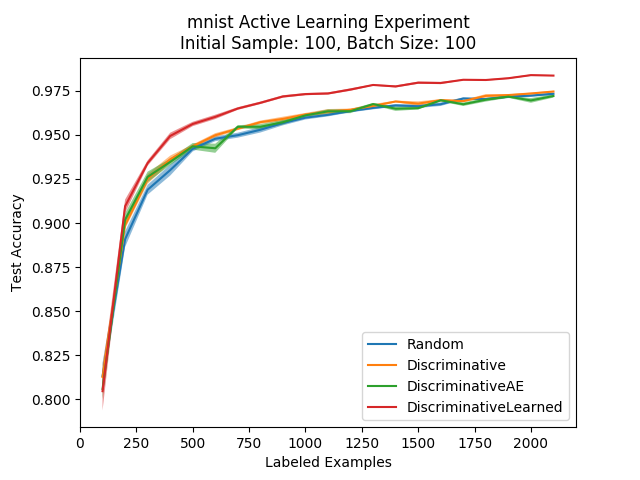
We can see from the first plot that it is clearly better to use the learned representation, which contains semantic information, as opposed to the raw pixel representation or the autoencoder one (even if that representation was good enough for the experiments with the linear model).
Sub-Batch Amount
Next, we turn to compare our method using different amounts of sub-batches (the amount of times we run the binary classification process until we query the entire batch). If we want to query 100 examples we can do anything between choosing the top 100 instances that are classified as “unlabeled” using a single classifier, up to iteratively running 100 classifiers and taking the top single instance at every time.
Intuitively, the larger the amount of sub-batches the better, since we have less of a chance of getting similar instances and we become more batch-aware. To check this intuition, we ran four different sub-batch amounts on the MNIST dataset and compared the results:
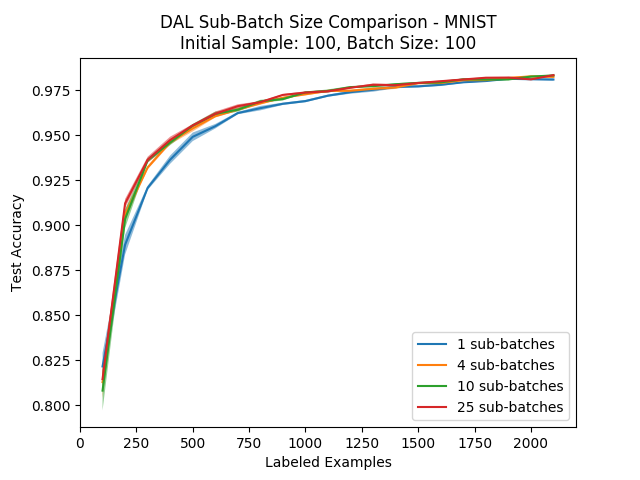
We can see that using a single sub-batch (getting the top-100 instances once) is definitely worse than using a few sub-batches, but as we increase the amount the improvement gets less significant. Still, it is reasonable to say that the more sub-batches we use the better our results will be, which leads to a tradeoff between running time and performance. Also, the more classes we have in our dataset (or more modes in our data distribution), the more we should expect this parameter to be significant…
As for the sub-batch amount that was used in the following experiments where we compared DAL to the other methods, we used 10 sub-batches on MNIST and 25 sub-batches on CIFAR-10.
MNIST & CIFAR-10 Comparison
Next, we move to comparing our method to all the other ones on MNIST and CIFAR-10. These plots are the ones presented in our paper. First, we will look at the results for the MNIST dataset, with a batch size of 10, 100 and 1000:
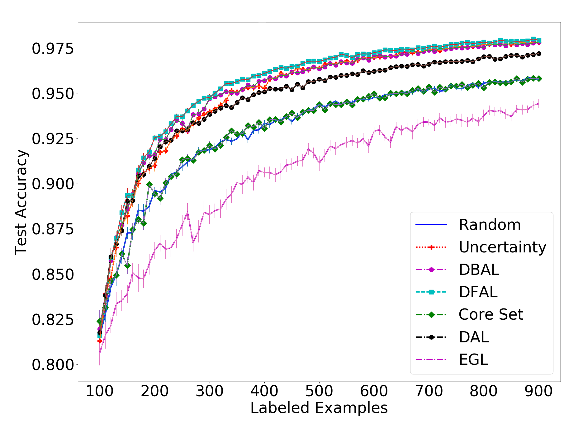
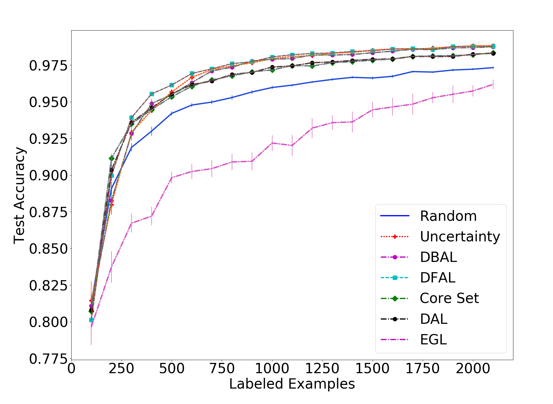
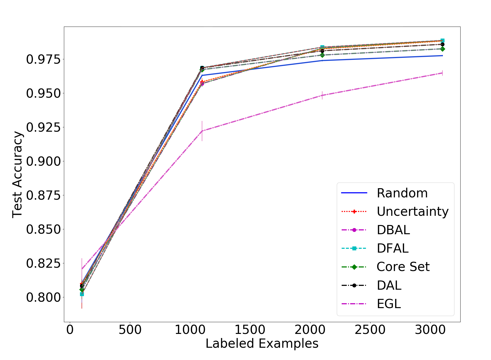
In the MNIST results we see our method being less effective than the uncertainty-based methods and the adversarial approach when the batch size is small. However, we do see that DAL is overall better than the core set approach, especially when there is a small batch size and the core set approach is reduced to being only as good as random sampling.
Next, we will look at the results on the harder CIFAR-10, with batch sizes of 1000, 5000 and 10,000:
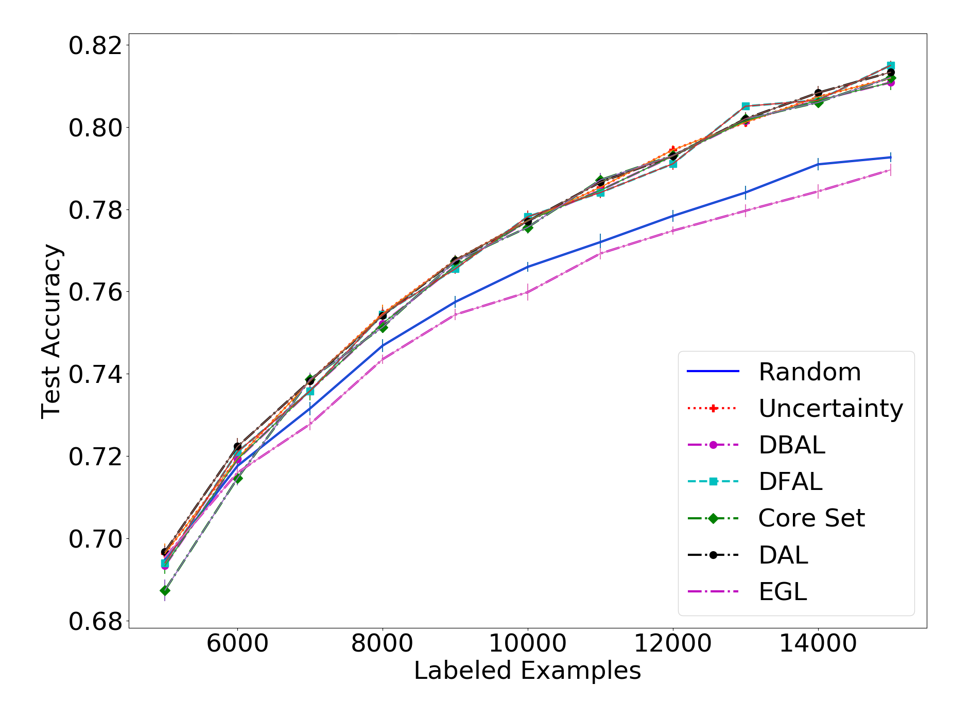
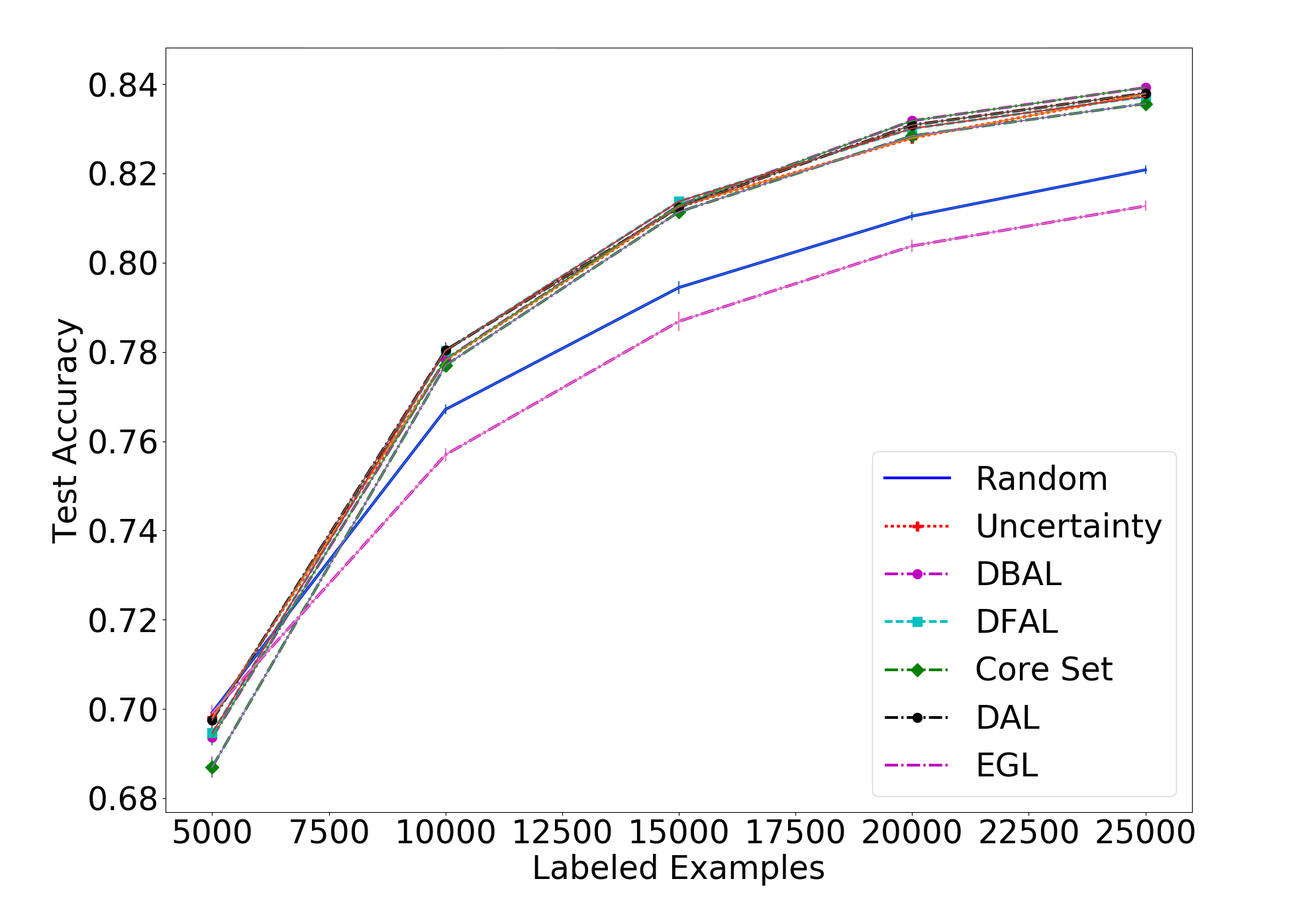
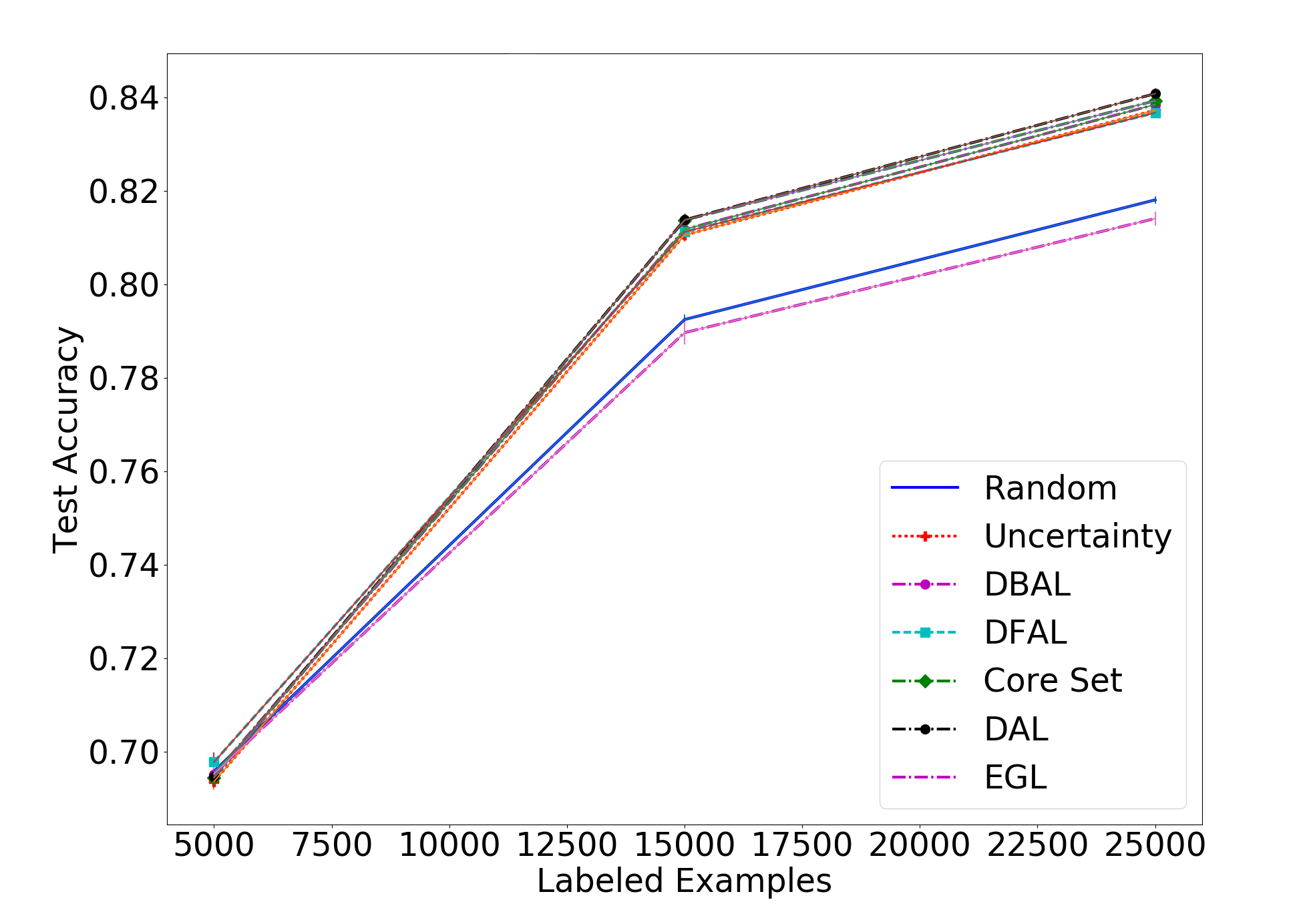
On the CIFAR-10 front, we see that our method is on par with the rest of the methods, having negligible differences to the others. While we obviously hoped to get a clear win for our method over the others, it is pleasing to see that for difficult tasks they all seem to perform similarly. Our method, while being very different from all others, performs on par with the rest.
Finally, let’s look at how our method looks in the label entropy metric against the other methods:
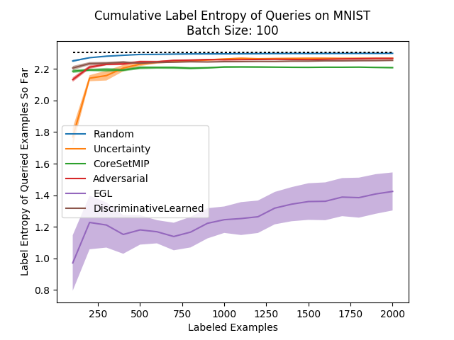
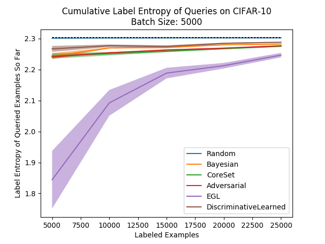
Seems relatively consistent with what we would expect… Our method has results which are higher than others while not beating their accuracy scores, but that’s not a problem since this measure is only a heuristic. We see our method leads to diversely labeled batches.
Implementation Details
The binary classification task we are trying to solve is very unbalanced since most of the time we’ll have an order of magnitude more unlabeled examples than labeled examples. This means we need to be careful in the way we train our neural network to make sure we don’t get a classifier that just thinks everything is “unlabeled”.
We found that there were two things that were crucial in this case. First, we need to make sure that the class weights are balanced, so that labeled examples will affect the loss function more than unlabeled ones. Second, we need to make sure the batch size is large enough so that we have labeled batches in every batch on average. Otherwise, the training process will have many gradients which lead the network to thinking all examples are unlabeled, and that’s a local minimum that could be hard to get out of. This means that if there are 10 times more unlabeled examples than labeled examples, you should aim for a batch size that isn’t much smaller than 64 to be on the safe side.
As for the architecture used for the binary classification, we chose to use a MLP architecture (a deep fully connected neural network) for simplicity and speed, and you may take a look at the code for the exact details which weren’t too important. We should note however that since we are basically trying to classify random labels, we’re asking the network to overfit a difficult classification task and so we shouldn’t use any form of regularization (no weight decay, dropout and so on).
Finally, to insure that our network isn’t overfitting the binary classification task too well (which would cause the sampling process to resemble random sampling), if the accuracy of the classifier goes over 98% we stop the training early (assuming we subsampled the unlabeled set to have 10 times the number of examples as the labeled set).
Attempt at a Stochastic Variant
As we said earlier in the post, we had a few ideas to try and make our algorithm more robust to outliers. Experiments we ran didn’t pan out, and one of them was the following:
We tried to use a stochastic decision rule instead of the hard one, by weighting the probability of choosing an example to be labeled in proportion to a function of the softmax scores of our binary classifier. The function we tried to test was the following, where we denote the predicted probability of being “unlabeled” as \(y(x)\):
In this way, the temperature parameter can help us decide how much we want to put an emphasis on the examples which are “unlabeled” with a high confidence. We ran this algorithm on a wide range of possible temperatures:
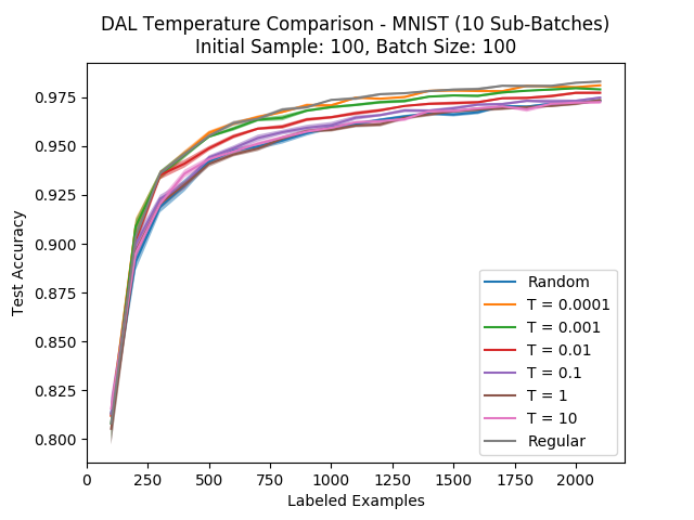
We can see that the smaller the temperature (the more we put an emphasis on the classifier confidence), the closer we are to the original algorithm. Also, the larger the temperature, the closer we are to random sampling. This is more or less what we would expect, but we also hoped that there would be some sweet spot in the middle of the temperature range where we perform better than the original algorithm, but that isn’t the case. We should say that we checked lower temperatures as well, but they begin to cause numerical problems…
A possible explanation here would be that while the two dimensional toy example gave us a certain intuition (susceptibility to outliers) that breaks down on real, high dimensional data. Regardless, seeing this caused us to stop persuing this direction…
Summary
In this post we introduced Discriminative Active Learning (DAL), a new active learning algorithm for the batch setting. We gave some intuition as to why the method should work, and presented the thought process and experiments we ran until we got our final algorithm.
We compared DAL to the methods we covered in the previous post and saw that it performs similarly to the core set approach, while being easier to implement and more scalable. We also saw that our method shares the task-agnostic nature of the core set approach, making it very easy to adapt to machine learning tasks which aren’t classification.
While we would have hoped to see our method beat all other methods, this isn’t really the case. Still, the results are on par with today’s state of the art which is pleasing. In the end however, when dealing with a real active learning task, we can’t recommend our method over good old uncertainty sampling, without running more experiments.
If you found DAL interesting and would like to read more about it and other theoretical motivations for it from domain adaptation and GANs, you’re welcome to read our paper.
In the next post we will conclude this blog series by quickly going over what we learned and highlighting what we think are the most important take home messages.