Comparing The Methods
In the previous post we surveyed some of today’s state of the art active learning methods, applied to deep learning models. In this post we will compare the methods in different situations and try to understand which is better. If you’re interested in our implementation of these methods and in code that can recreate these experiments, you’re welcome to check out the github repository which contains all of the code.
Disclaimers
Before we get into the experimental setup and the results, we should make a few disclaimers about the experiments and active learning experiments in general. When we run active learning experiments using neural networks, there are many random things that affect a single experiment. First, the initial random batch strongly affects the first batch query (and subsequent batches as well). Next, the neural network which trains on the labeled set is a non-convex model, and so different random seeds will lead to different models (and representations). This in turn causes another problem - when we want to evaluate the test accuracy of a labeled set gathered by an algorithm, different evaluations (which require training a neural net on the labeled set) will lead to different test accuracies…
All of these random effects and others mean that we should be extra careful when running these kinds of experiments. Sadly, most papers on this subject do not specify their complete experimental setup, leaving many things open to interpretation. Usually we are lucky to get anything other than the model and basic hyper parameters that were used, and this means we had to try and devise a setup which is as fair as possible to the different methods.
Another important parameter for the experiments that changes between the papers is the batch size. As we saw in our last post, having a large batch means that there is a bigger chance of the chosen examples being correlated and so the batch becomes less effective at raising our accuracy. Not surprisingly, papers that propose greedy active learning methods use a relatively small batch size while papers that propose batch-aware methods use a very large batch size. These choices help in showing the methods’ stronger sides, but they make comparing the methods harder. We compared the methods in a wide range of batch sizes to be as fair as possible.
As you will see, our experimental results are different from some of the results reported in the papers. When these differences occur, we will point them out and try to give an explanation, although in some of the cases we won’t have a good one.
Experimental Setup
So, after that long disclaimer, how did we choose to setup the experiments?
A single experiment for a method runs in the following way:
-
The method starts with a random initial labeled set and a large unlabeled set.
-
A neural network is trained on the labeled set and the resulting model is handed over to the method. The model architecture and hyper parameters are the same for all the models.
-
The model accuracy on a held-out test set is recorded. This test set is the same for all the experiments and methods.
-
The method uses the model to choose a batch to be labeled and that batch is added to the labeled set.
-
Repeat from step 2 for a predetermined amount of iterations.
We run 20 experiments for every one of the methods and then average their accuracy in every iteration over all the experiments. The plots in this post present the average accuracy for every iteration, along with their empirical standard deviations.
We’ll now move to some final nitty details of an experiment.
Initial Labeled Set
The initial labeled set has a big effect on the entire experiment. To make things fair, we used the same initial labeled set for all the methods. For example, if we ran 20 experiments for all of the methods, there would be 20 initial labeled sets that would be the same for all the methods. This insures that we control for the effects of the randomness of the initial labeled set.
Training a Neural Network on the Labeled Set
As we said, the neural network training can have different results on the same labeled set. We tried experimenting with many forms of early stopping and running several evaluations and taking the best one, but these didn’t seem to work very well (mostly due to the difficulty of stopping the training at the right time).
The method we found that works best was to train a neural network only once, but to train it for much longer than necessary while saving the weights during training after every epoch where the validation accuracy has improved or stayed the same. The validation set was always a random subset of 20% of the labeled set. This allowed us to not worry about early stopping issues and made sure that we got the best (or close to the best) weights of the model.
This does not completely control for the randomness of the neural network training, but we found it reduces it quite a bit and we are able to deal with the randomness by running several experiments and averaging over them…
Comparison on MNIST
We start with a comparison on the MNIST dataset. The architecture we use here for all the methods is a simple convolutional architecture (the LeNet architecture). For a detailing of the hyper parameters you’re welcome to look at our code. The batch size we used here was a batch size of 100, and an initial labeled set of size 100 as well. For additional batch sizes you’re welcome to look at our next post.
The methods we compared are random sampling, regular uncertainty sampling (using the softmax scores), Bayesian uncertainty sampling, Adversarial active learning, EGL, core set with the greedy algorithm and core set with the MIP extension.
First, let’s compare the methods separately against random sampling, the usual baseline.
Uncertainty Sampling Methods
We’d like to see how much the Bayesian approach to uncertainty estimation in neural networks improves performance in active learning, in comparison to the regular uncertainty sampling which simply uses the softmax scores. In the following plot we compare the different methods, along with the different possible decision rules (top confidence and max entropy):
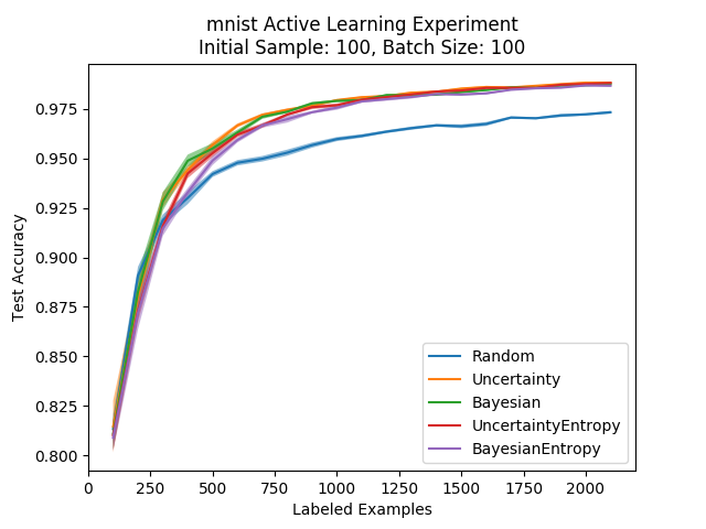
We can see that the differences are more or less negligible, with all of the alternatives performing much better than random sampling. The only real difference we can note is that the top confidence decision rule is better than the entropy one at the initial stages of the active learning process. These results are more or less consistent with what is presented in the paper.
Following this comparison, we will only use the top confidence decision rule for our comparisons to make the graphs more readable.
Adversarial Active Learning
We have only one formulation of this method that we checked, which corresponds to the formulation in the paper. Let’s see how it compares to random sampling:
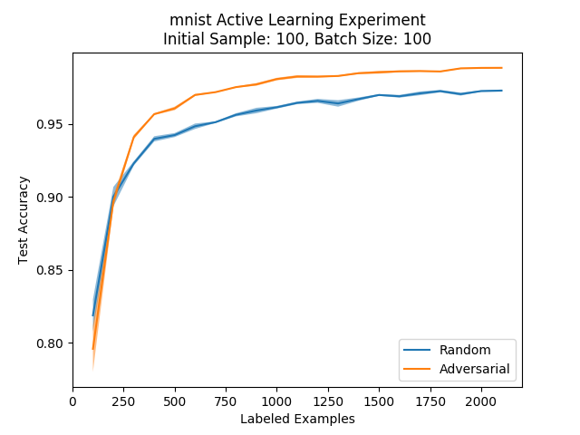
We can see that the adversarial approach beats random sampling by a significant margin.
Core Set Methods
Next, we compare the greedy core set method with the MIP formulation. As detailed in the core set paper, adding the MIP formulation increases the running time of the core set algorithm considerably (and we saw this in our experiments as well). However, it does improve the performance:
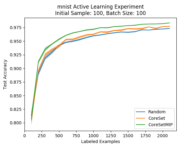
Well, we can see that the MIP formulation has a very positive effect from very early on in the active learning process, which is very nice to see. This improvement is consistent with what was reported in the core set paper, even though we couldn’t use the entire unlabeled set like they did. We should note that while we haven’t explored this idea enough to make any definitive claims, we feel that this improvement is brought on mainly due to the robustness to outliers of the MIP formulation.
So, we can conclude that if you are OK with waiting a bit before getting the next batch of examples to be labeled, and if you have the resources to solve a MIP optimization problem with many variables, it is worth it to use the MIP formulation. Still, it’s nice to see that the method beats random sampling even in its greedy formulation, although the difference isn’t very large. This is mostly due to the relatively small batch size, which means the method’s batch-aware nature is less present.
EGL
We implemented EGL and compared it to random sampling:
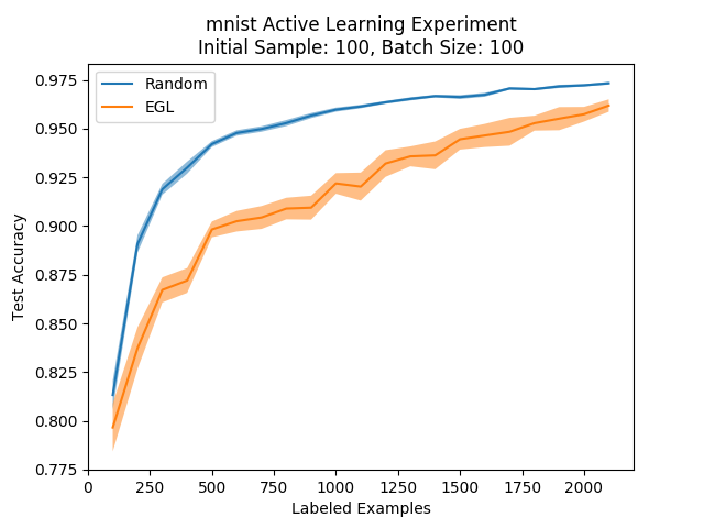
Oh. This looks bad.
This was also the case in the adversarial paper when they tried to compare their method to EGL, but the EGL paper shows great improvements against both random sampling and other methods, so what happened?
We’ll explain what we think happened later in the post.
Full Comparison
So how are the methods ranked against each other on the MNIST dataset?
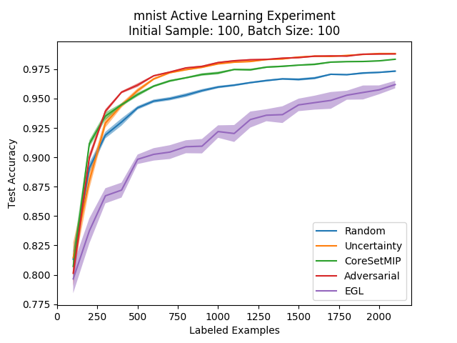
Interestingly, we see that the adversarial approach is on par with the uncertainty-based approach after a few iterations. A possible explanation for this (which we’ll see more evidence for later) is that the adversarial approach behaves similarly to the uncertainty-based methods. We saw that in the linear case the margin-based methods are the same as the uncertainty ones, and the adversarial approach is a margin based approach, so maybe this extends to neural networks…
While the adversarial and uncertainty methods look similar, we see that the core set approach is different from them (and a bit worse on MNIST). This can possibly be attributed to the small batch size, since the core set approach is designed for large batch sizes to take advantage of having a batch that is as diverse as possible.
But all of this is just a comparison on MNIST, the most worn out dataset in history. We’d like to compare the methods on more realistic datasets and with a larger batch size, which simulates real-life active learning problems better. For that we turn to an image classification dataset that is only a bit less worn out - CIFAR!
CIFAR-10 Comparison
CIFAR-10 is an image classification dataset with 10 classes. As opposed to the MNIST dataset, the images here are RGB and a bit larger (32x32). This task is harder and so we need a better, deeper architecture to solve it. We chose to follow the lead of the core set paper and use the VGG-16 architecture, a deep convolutional neural network which is rather popular in general as a pre-trained feature extractor. We used a much larger batch size this time - a batch size of 5000, along with an initial sample of 5000 examples.
We chose this batch size both because it was the setting in the core set paper, and because it gives us a view of a batch size that is orders of magnitude larger than the one usually used when comparing these methods. We also believe that this batch size is much more realistic for industry applications, where the datasets are usually very big and the labeling is paralleled.
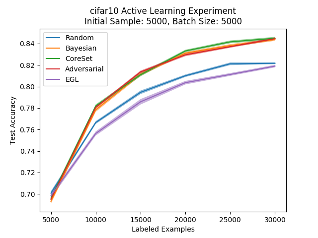
So, we see that in CIFAR-10 there is still a clear advantage for the different methods against random sampling. Also, we can see that the tested methods perform more or less the same and that their differences are negligable.
We can take a couple of things away from these results. First, the success of these active learning methods isn’t restricted to toy problems like MNIST - the methods are clearly an improvement over random sampling even in CIFAR-10. Second, we see that when we raise the batch size to 5000, the greedy methods continue to perform well which isn’t necessarily what we see in the core set paper or what we would intuitively expect. However, we do see that the batch aware methods perform much better in a larger, more realistic setting.
As for how all these results compare to the literature, we should point out one difference that keeps coming back - uncertainty sampling gives us consistently good results while it gives weaker results in the papers. The Bayesian active learning paper doesn’t provide comparisons to the regular uncertainty sampling, while the adversarial approach paper seems to suggest that the uncertainty sampling method (along with the Bayesian adaptation) perform worse than random sampling for most of the active learning process, a result that is far from what we saw here. In the core set approach’s paper when comparing on CIFAR-10 data we also see that uncertainty sampling and the Bayesian approach are more or less on par with random sampling, which is also not the case in our experiments. This is quite surprising since the uncertainty sampling method is very simple and easy to implement, but these differences could be due to differences in the experimental setup between the papers and us.
Batch Composition & Label Entropy
In this section we’ll try to learn more about the behavior of the algorithms by looking at how a queried batch is distributed across the different classes. We did this both as a sanity measure and to try and understand why EGL’s results were so bad, under the hypothesis that it is because there is very high correlation between the examples that are queried by EGL.
To summarize the distribution of labels in the examples that were queried with a single scalar, we’ll define the notion of “label entropy”. The label entropy of a set of \(M\) examples will be the entropy of the empirical distribution of labels in the set. Mathematically, this can be written as:
Like in regular entropy, a high label entropy corresponds to higher uncertainty on the labels in the set. Since we want active learning methods to create a labeled set that is relatively diverse and represents the full distribution well, we should expect a good active learning method to create a labeled dataset which has a similar label distribution as the full dataset. Since our full dataset has the same number of images for every label (maximal entropy), we would say that as a rule of thumb, higher label entropy during the active learning process is better.
It isn’t very difficult to record this label entropy in our experiments, and so we recorded the entropy of the different algorithms. In every iteration of the experiment we calculated the label entropy of all the examples queried so far, and in the following plot we can see the results averaged over several experiments (the dotted black line is the maximal entropy over the number of classes):
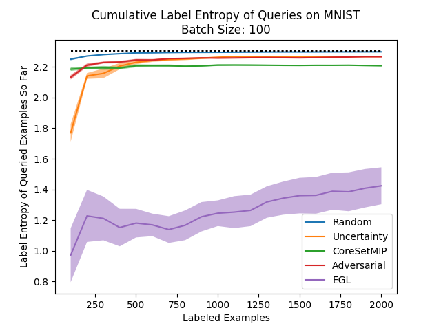
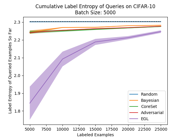
This is very interesting - except for the random sampling which has the highest label entropy (unsurprisingly), we see a very strong correlation between the accuracy ranking of the methods and their label entropy! This is quite pleasing and shows that this measure can possibly be used as a proxy for the success of an active learning method in practice. If the method you’re using has a label distribution that is far from the label distribution you expect for your data, you may suspect that the method isn’t working very well…
Another interesting thing to note here is the label entropy of EGL which is much, much lower than all the others, and barely improves during the process. This confirms our suspicions - EGL continuously queries examples from the same few classes and does not lead to a balanced labeled dataset. This explains the poor performance it had during our experiments…
But the EGL paper showed great results, so what happened?
Remember that the team at Baidu implemented EGL as an active learning method for speech recognition using RNNs, and our experiments were all on image classification tasks using CNNs. The two architectures are very different and so it is quite plausible that the architectures have gradients that behave differently. It is also possible that there was a difference in the regularization used on the model, which affects the gradients. With all these differences, it isn’t surprising that the gradients will behave differently between the experiments, and because EGL is based on the expected gradient norm, it isn’t surprising that we will see this difference in performance.
Checking that our suspicions are correct regarding the difference in gradient behavior is interesting, but is outside the scope of this project…
Ranking Comparison
Another interesting way we can compare methods is used in the EGL paper, and we will use it here too. We can look at the way each method ranks examples in the unlabeled set from high score to low score (applicable only to the greedy methods) and try to look at the rankings. Similar methods should rank the unlabeled set in a similar way, so that if we plot the rankings one against the other we should expect them to more or less line up on the diagonal of the plot. On the other hand, methods which are very different should have plots that are all over the place.
We’ll start by comparing two methods which we should expect to be similar - uncertainty sampling and Bayesian uncertainty sampling. Note that we’ve ordered the ranking such that those who are ranked first (bottom and left) are those that will be selected first (ranked most informative under the query strategy) and we’ve normalized the ranking to be between 0 and 1:
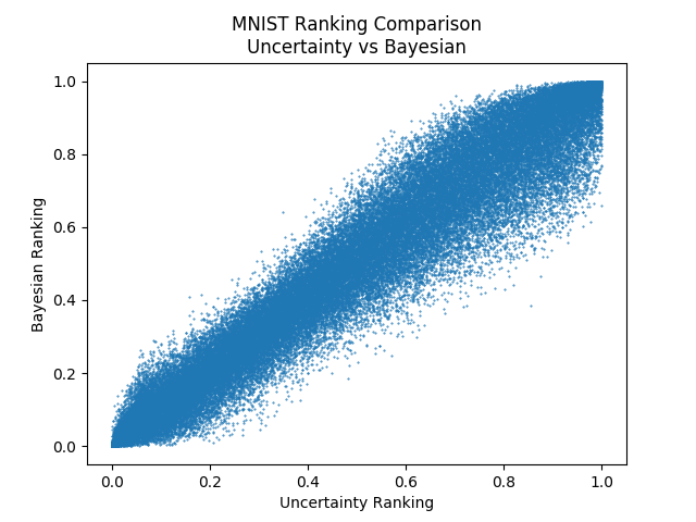
Indeed, we got that the two methods rank the unlabeled examples in a very similar way. Next, we can have a look at the adversarial method. We saw in the comparison on MNIST that the methods perform similarly and they’re intuition is similar, so do they rank the unlabeled set similarly as well?
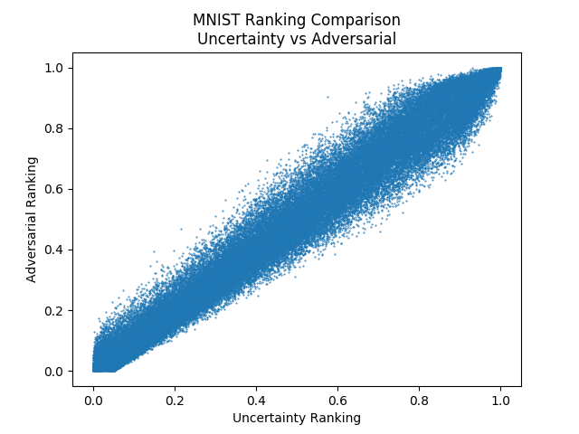
It seems so!
While the two methods are very different in what they do, the eventual results are very similar. A comparison of the adversarial approach to Bayesian uncertainty sampling looks basically the same.
Finally, we’ll have a look at EGL compared to uncertainty sampling. We expect there to be little correlation since we saw EGL selects examples predominately from the same class…
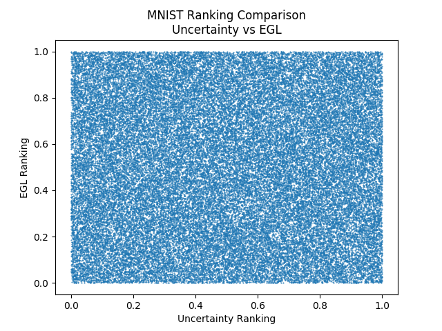
No correlation at all.
Summary
In this post we empirically compared the different methods that we detailed in the last post, using the MNIST and CIFAR datasets. We saw the effect of the batch size on the different methods and reviewed two additional interesting ways to compare active learning methods - the label entropy and the ranking comparison.
We also saw that the methods can be sensitive to the actual objective we are optimizing, along with the network architecture. This is especially true for methods like EGL, which use the model’s gradient as part of their decision rule (and it might also be true of the adversarial approach for this same reason).
Overall, while the different methods perform differently in different situations, it doesn’t seem like any of them really beat the good old uncertainty sampling. This comes in contrast to what is shown in the different papers, but we stand by our results as we feel we have taken great care to run fair comparisons and experiments.
In the next post, we will review the work we did on developing a new active learning method - “Discriminative Active Learning” (DAL). The method gives results which are comparable to the other methods detailed here, but we weren’t able to clearly beat any of them. Still, we feel the method and thought process is of interest. If you would rather skip ahead, the post after that concludes this review of active learning.