Introduction to Active Learning

The Basic Setup

The idea of AL is, instead of just giving the learner a lot of data to learn from, to allow the learner to ask questions about the given data. In particular, the learner gets to ask an oracle (some human annotator) about the label of certain instances that are currently unlabeled. If the learner asks smart questions, he might be able to get examples that are very informative and reach a high level of generalization accuracy with a much smaller labeled dataset than he would have if that dataset had been created using random sampling.

The classic motivating example would be the following 2-dimensional data, which we are trying to separate using some linear classifier:

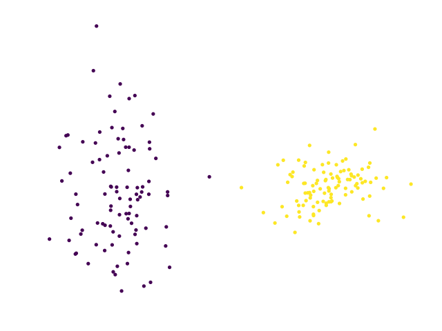
Clearly, we can separate these two blobs linearly using a vertical decision boundary, but this is not so obvious when we only get to see the labels for a small number of these points. Given the wrong subset of these points, we could choose a decision boundary that fails to separate the data correctly…

Let’s compare random sampling to an active learning algorithm called “uncertainty sampling” (which we will explain later). Both algorithms get one initial labeled point from each blob (marked in red) and sequentially ask for the label of an additional point (marked in green). In every iteration, we train a linear SVM classifier on the labeled set:

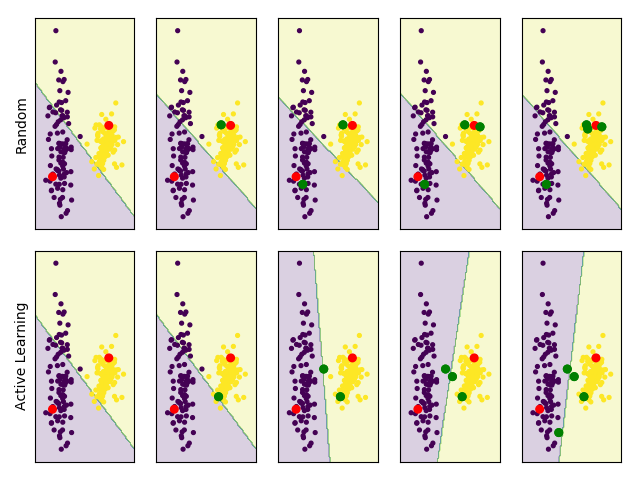
The two initial points give us a slightly tilted decision boundary that doesn’t separate the data well. We can see that random sampling chooses points in the dense yellow blob, which don’t give us much information and so the decision boundary stays more or less the same, and we aren’t able to separate the data well. On the other hand, the active learning algorithm is able to choose points which are very informative and quickly gets to the correct decision boundary.

This is the promise of active learning - reduce the number of samples needed to get a strong classifier by choosing the right examples to label.

Possible Scenarios

There are three main scenarios where active learning has been studied. In all scenarios, at each iteration a model is fitted to the current labeled set and that model is used to decide which unlabeled example we should label next.

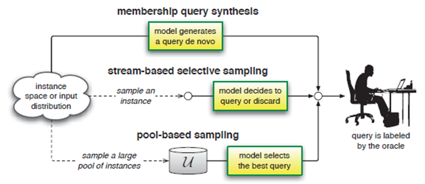
The first scenario is membership query synthesis, where the active learner is expected to produce an example that it would like us to label. This scenario requires that the model will be able to capture the data distribution well enough to create examples which are reasonable and that would have a clear label - if we are classifying images and the learner produces an image that is pure noise, we won’t be able to label it… Due to this limitation, people grew less interested in this scenario.

The next scenario is stream based, where the learner gets a stream of examples from the data distribution and decides if a given instance should be labeled or not.

The third scenario, and the one we will focus on here, is pool based active learning. In this scenario the learner has access to a large pool of unlabeled examples and chooses an example to be labeled from that pool. This scenario is most relevant for when gathering data is simple (scraping images/text from the web for instance), but the labeling process is expensive.

Query Strategies

Most active learning algorithms start the same way - we fit a model to the labeled set and so we have access to \(\hat{P}(y|x)\). Where they differ is how they choose the example to query, given the trained model - the query strategy. There are many possible heuristics for choosing the best example to query, and we’ll detail the most common methods.

Uncertainty Sampling

This is probably the simplest and most straightforward idea - make the learner query the example which it is least certain about. For binary classification, this boils down to choosing the example on which the model’s prediction is closest to a coin toss. When we are working in a multiclass setting, there are different ways of defining uncertainty. The most popular ways are either top confidence or maximum entropy.

Top confidence looks only at the label that the model would have predicted for the example and asks how much probability was given to said label. It then chooses the example where the top label had the smallest probability. This is the simplest extension of the binary classification setting, and leads to the following decision rule:

$$\underset{x}{\mathrm{argmin}}\,\underset{y}{\mathrm{max}}(\hat{P}(y|x)))$$

Maximum entropy uses the label distribution’s entropy as a measure for the uncertainty of the model on an example. This considers the probabilities of all possible labels. The resulting decision rule then becomes:

$$\underset{x}{\mathrm{argmax}}\,-\sum_{y \in Y}\hat{P}(y|x)log(\hat{P}(y|x))$$

When we are talking about linear classifiers like in the blob example above, choosing according to the uncertainty sampling heuristic is the same as choosing the sample closest to the decision boundary. In the blob example we used uncertainty sampling as our query strategy, and we can clearly see that the chosen examples really are those that are closest to the boundary. This margin-based approach is equivalent to the uncertainty approach only for linear classifiers though, and we’ll address this difference in the next post when we look at active learning for neural networks…

So, all this sounds reasonable, but is it any good?

To check, we can compare the uncertainty sampling method to the regular random sampling method on a simple binary classification task. We’ll try to separate MNIST digits, where one class is the digit “3” and the other is “5”. Starting with a single labeled example from each digit, we will use uncertainty sampling to choose the next example to label. The model we will fit in every iteration will be a logistic regression model. These are the results averaged over 10 experiments:

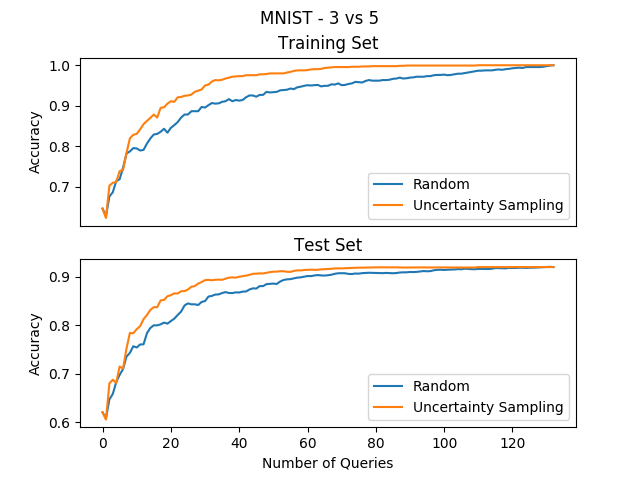
Awesome! With a simple heuristic we were able to get a perfect accuracy after only querying ~50 examples, while the random sampling method still hasn’t converged after over 100 examples… So we reduced our labeling costs by over 50%.

Query By Committee

The second heuristic that was very prominent in the early days of active learning research is QBC. The idea here is similar to the uncertainty sampling idea but extended to ensembles - instead of looking at the uncertainty of a single model on the unlabeled set, we’ll train several different models on the labeled set and look at their disagreement on examples in the unlabeled set. The intuition here is that if our ensemble disagrees on a specific example, then querying that example’s label should be more informative because our collective model is uncertain about it.

QBC also has another interpretation though. The model which we are trying to learn comes from a certain hypothesis class (for example, the class of all linear classifiers). When we have a small number of labeled examples, there could be many possible models that fit the data, but some of them might not generalize well. If we look at our ensemble as a set of models from different viable parts of the hypothesis class (also called the “version space”), then choosing the example with the biggest disagreement corresponds to making the current version space as small as possible. This can help us zero in on the right hypothesis using a small number of labeled examples, like we want.

In the same way that we can define different measures for “uncertainty”, we can also define different measures of “disagreement”. An example of such a measure which corresponds to uncertainty sampling’s maximum entropy measure is the “vote entropy”. Here, we count the votes for every possible label and normalize so that it’s a distribution and look at the entropy. If \(M\) is the size of our ensemble, the decision rule we end up with is:

$$\underset{x}{\mathrm{argmax}}\,-\sum_{y \in Y}\frac{Votes(y)}{M}log(\frac{Votes(y)}{M})$$

To check if QBC is any good on the binary MNIST example, we can use 10 SVMs with different regularization coefficients to get different viable models for the labeled set, and then use their disagreement to choose the next example to label. Running the experiment gives us the following results:

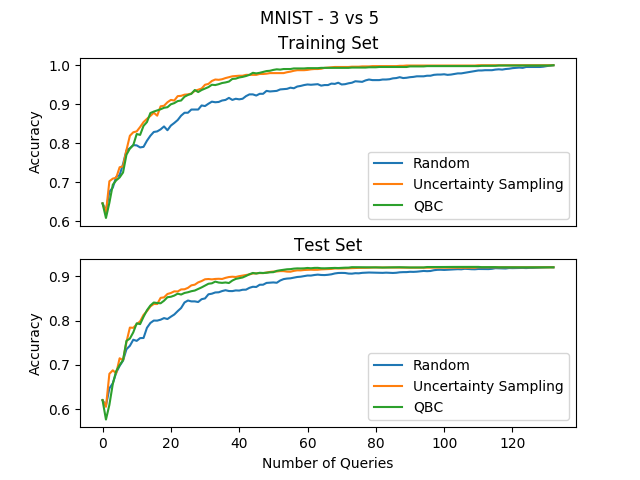
Great results again!

Other Strategies

The two methods above are by far the most popular methods for the classical AL setting, but there are many other methods which were developed over the years. Here are two examples:

• Expected Model Change is an approach which tries to query the examples which we expect to cause the greatest change to our model. For models that we can calculate the gradients to (neural networks for example), a possible approach can be to choose the example with the largest expected gradient length (EGL), where the expectation is over the probabilities that the model gives to the labels. The decision rule for EGL is:

$$\underset{x}{\mathrm{argmax}}\,\sum_{y \in Y}\hat{P}(y|x)||\frac{\partial l(x,y)}{\partial \theta}||$$

• Density Weighted Methods tries to query examples which have both a high uncertainty and which are “representative”, meaning they are in dense regions of the data manifolds. This method avoids choosing examples which are outliers, even if they have a high uncertainty, under the assumption that outliers give us less information on the data distribution.

Summary

In this post we learned about the basics of active learning. We saw that if we extend the supervised learning model to allow the learner to query specific examples to be labeled, we can significantly reduce the number of samples needed to get the desired accuracy. We also went over the classic query strategies which achieve that improvement.

But the active learning scenario we introduced has some big limitations if we want to really implement it in real life applications. Our scenario assumes that the learner asks for the label of a single example, but that means that we need to wait for our neural network to converge for every single query, and that can take a long, long time. Also, it means we can’t use many human annotators, which is the strength of services like Mechanical Turk.

In the next post, we’ll dive into the more practical scenario for active learning - Batch Active Learning. We’ll understand the new challenges it poses and cover today’s state of the art query strategies for deep learning.