A Primer on Implicit Regularization
The way we parameterize our model strongly affects the gradients and the optimization trajectory. This biases the optimization process towards certain kinds of solutions, which could explain why our deep models generalize so well.
In the last blog series, we saw how a deep parameterization can cause the gradients of our model (a quadratic neural network) to be non-convex and hard to manage. That led us to try and develop algorithms for optimizing the network in a linear space, to get all the good theoretical guarantees that classical convex optimization gives us for SGD. We saw that it’s difficult to get these algorithms to work, and even then they’re hard to generalize to large neural networks.
This time, we will lean into the non-convexity and surprising dynamics of these parameterizations. We will analyze how different parameterizations of the same function lead to wildly different optimization dynamics, and how this sort of analysis can help us understand how neural networks generalize so well. Since the last blog series was a bit long, no prior knowledge is assumed.
All of the plots in this post can be recreated using the jupyter notebook here.
- Introduction
- The Toyest of Models
- The Interplay of Parameterization and Gradient Dynamics
- Multiple Zero-Loss Solutions
- Conclusion
- Further Reading
- Footnotes & References
Introduction
One of the big questions in theoretical ML today is to try and explain how it is that neural networks generalize so well to unseen examples while being so expressive as a model. For many difficult tasks, neural networks can memorize random labels, more or less meaning that we shouldn’t expect them to be able to generalize to new examples. There is an infinite number of solutions for these datasets that get a loss of zero (ERM solutions), some of these generalize very poorly - if we chose one of these at random, we shouldn’t expect it to generalize.
But we aren’t choosing a solution at random - we use a specific algorithm for finding the solution, and that algorithm biases us towards a specific kind of solution out of all the possible ones. There are types of solutions SGD favors, and characterizing them may help us explain why neural networks generalize so well.
This is the premise of the theoretical study of implicit regularization as a way of explaining generalization in neural networks. We want to see how the interplay of gradient based optimization and the parameterization of the function we are optimizing affects the kinds of solutions we get from our model. In this blog post we will use toy models to get a sense of how much of a difference this implicit regularization has on the solution, and get a relatively gentle introduction into this very interesting field.
The Toyest of Models
While there’s been a lot of work in recent years on implicit regularization in relatively complicated models, we will look at a very simple model - a linear 2D model. This will allow us to visualize the gradients of the different parameterizations while still seeing all of the interesting phenomena that exist in larger models.
Our model will be parameterized by , and there will be an optimal set of parameters that we wish to learn using gradient-based optimization. Our loss function will be the squared loss1:
This loss is simply the squared distance to some optimal set of weights (which we want to learn). This setting is a simple one, but we will see interesting effects as we change the parameterization of our model. There will still be a that is equivalent to our model, but we will be optimizing over slightly different parameters each time.
The Interplay of Parameterization and Gradient Dynamics
We are going to explore how the gradient dynamics of our model behave in different conditions, so let’s remember how to calculate the gradient of our weights. For our loss function , the weights move in the negative direction of the gradient (as in gradient descent):
However, things look a little different when we play around with the parameterization. Instead of optimizing over , we can parameterize using an additional parameter, , and optimize over that. To make things clear, let’s look at an example - we can define in the following way:
Note that we didn’t really change anything - any function that we could have expressed with can still be expressed with an appropriate . While this change seems innocent and harmless (and redundant), it affects the gradients of our model. Since every set of parameters can be described by a set of parameters, we can compare the two cases on the same footing. On the one hand, we will look at the gradients of the original model, when we are optimizing over . On the other hand, we will look at how the gradients over change , the corresponding model to the given parameters.
Let’s look at the above example for and derive the gradient:
First, we need to calculate the gradient of . We can do this by using the chain rule over :
Now that we know how changes according to the gradient of the loss, we can ask how changes as changes. We can calculate this by applying the chain rule a second time:
Finally, we can invert our formula for to get . We can use this to describe as a function of :
Writing the gradients only as a function of the shows us that they are surprisingly different from the original gradients - the values of that we optimize are now weighted by the current value of . We should expect that values of that are close to will change very slowly, while large values should change rapidly. This is reminiscent of the exploding/vanishing gradient problem of deep neural networks, and it is basically a toy version of it - optimizing over a product of linear parameters causes the gradient’s norm to be strongly dependent on the current values of the parameters.
We can follow the above procedure for a general , to get a general formula for :
Now that we have a basic picture of the relevant concepts, we can start playing around with different parameterizations and make some nice visualizations.
Playing Around With Parameterizations
The nice thing about having a 2D model, is that we can plot the gradient in every point and visualize the gradient field over the loss surface. We can start simple, with the gradients over the original parameters:
For every , we will plot the negative gradient with respect to the loss. Because the size of the gradients will vary a lot in our plots, we will only focus on the direction of the gradients and plot all of them in the same size. For all of our plots in this section we will use the same optimal parameters , marked using a green dot in the plot:
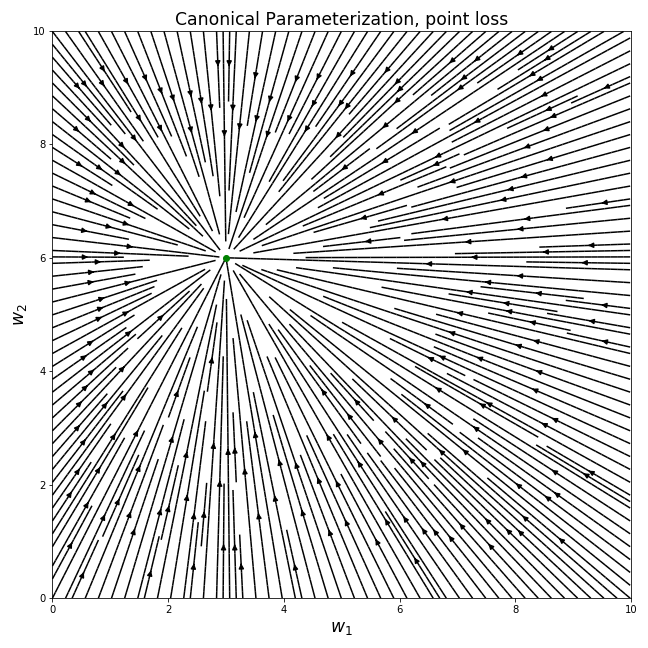
Every point in the above plot corresponds to a possible model (a set of parameters) - the axis describes the parameter and the axis describes . Every point has a line that crosses it, describing the direction of the gradient at that point, . Overall, this plot can be seen as an approximation2 of the optimization trajectory of gradient descent - if we initialize our model with some , we can follow the line from that initial point to to see the trajectory that gradient descent takes.
Perhaps unsurprisingly, optimizing the squared loss with gradient descent moves the parameters in the Euclidean shortest path to the optimal solution. This is one of the nice things about optimizing linear models which we explored in previous posts. However, as we’ve said, the gradient field looks quite different for different parameterizations…
“Deep” Parameterization
The example parameterization we saw before is a special case of a “deep” parameterization - instead of a shallow linear model, we have the parameters raised to the power of the “depth”. You can think of this parameterization as a deep neural network without activation functions, where the weight matrices are all diagonal and weight-shared.
For a depth model, we parameterize w in the following way:
Calculating the gradients as we did before, we get the following formula:
As before, we can plot the gradient field to see how the parameters move under gradient descent. We will focus on the positive quadrant of the parameter space, to avoid having to deal with even values of N where w can’t be negative under this parameterization:
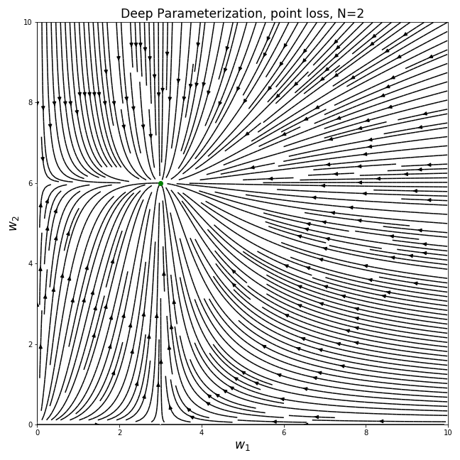
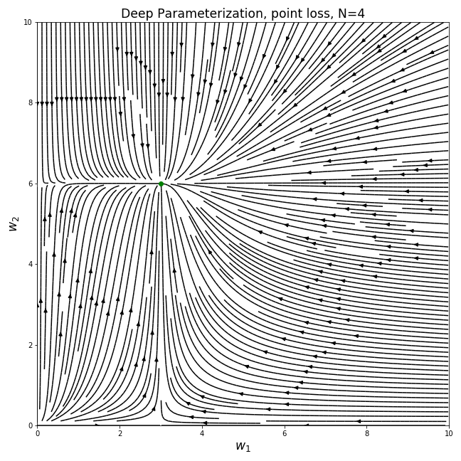
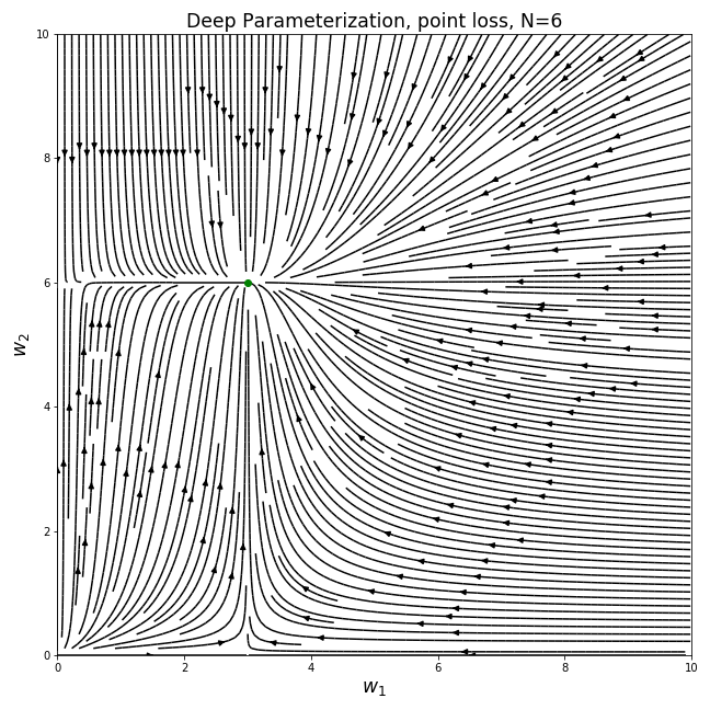
Immediately we see that these gradient fields are completely different than the previous one - the parameters no longer move in straight lines and they don’t take the shortest path towards the optimal solution. We see that when the values of the two current parameters are different, the gradients become biased towards the direction of the larger value.
Assuming we initialize the model with small random values (as is the case in deep learning), the trajectory follows a “rich get richer” dynamic - the larger value converges much faster than the small one. This sort of dynamic leads to the model being sparse for a large portion of the optimization trajectory. In the extreme cases, the values are more or less learned one by one.
We see interesting phenomena for deep models, and a reasonable thing to ask is what happens when we keep increasing …
“Infinitely Deep” Parameterization
We could ask how the dynamics of the deep parameterization will look like for . Surprisingly, this behavior happens when we parameterize our model with an exponent:
The gradient field in this case is indeed a limiting behavior of the deep parameterization:
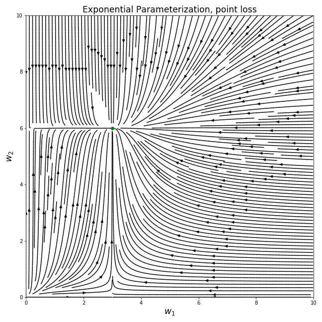
Let’s look at another parameterization - we tried a toy deep parameterization using a larger power than , let’s try a fractional power as a toy “anti-deep” model.
“Anti-Deep” Parameterization
If large positive powers bias us towards sparsity, do fractional powers do the opposite?
For a depth model, we parameterize w in the same way as before, to get us the following gradient fields:
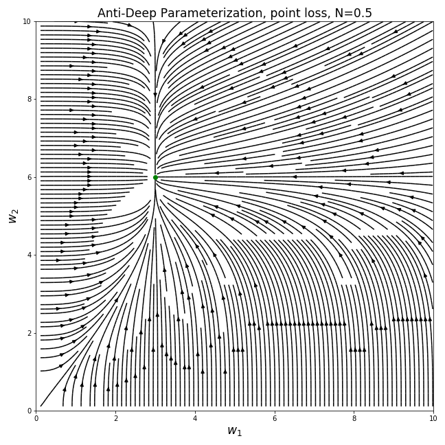
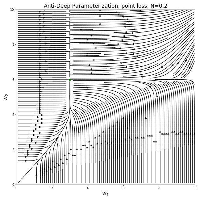
Interestingly, the behavior of the gradients are indeed opposite to the deep parameterization. Since the gradients are weighted by the inverse of the current weights, larger weights lead to smaller gradients and the optimization process, when initialized with small values, is biased towards having values of similar sizes. If the deep parameterization is of low norm for most of the optimization process, this parameterization has low norm.
Finally, we can’t look at 2D parameterizations without exploring one of the classics…
Polar Parameterization
We can use polar coordinates to parameterize our model in the following way:
The gradient field for this parameterization:
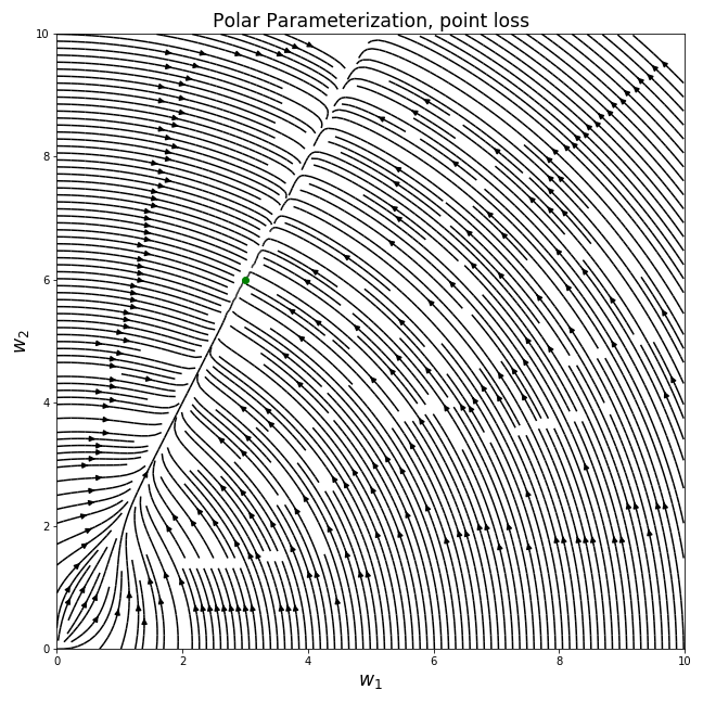
This plot is quite different than the previous ones, and it’s hard to define a clear bias for the path that the model takes until convergence. Note how for small radii the gradients are more inclined to increase the radius, while for radii larger than 1 the gradients have a much stronger angular component. This is caused by the fact that the angular gradient is weighted by the radius, and so we get an angular behavior similar to our deep parameterization.
All of these plots should drive the point home that small changes to the parameterization of the function that don’t affect the expressiveness of our model can lead to completely different optimization behavior. Still, you may ask why we should care so much about the optimization trajectory when all of these models eventually converge to the same solution. Great question.
Multiple Zero-Loss Solutions
While the demonstrations above were for a toy model and a very simple loss function, and so all of the parameterizations converged to the same solution, real models (and neural networks especially) can have many different zero-loss solutions that generalize differently to unseen examples. We should expect parameterizations with different trajectories to converge to different solutions, which means that there would be parameterizations that generalize better than others, for the same class of functions.
To illustrate this, let’s look at a different loss function that has multiple solutions. Instead of the squared distance from an optimal point, we will use a loss that is the squared distance from an optimal line. For an optimal line defined by the following equation:
Our loss function will be the squared distance from that line:
Note that this loss isn’t unrelated to real-life models. Up to a scalar multiplication, it is equivalent to the squared loss over a dataset with a single example with the label . Since we have more parameters than examples ( vs ), we can expect there to be multiple optimal solutions (infinite in our case). It is then reasonable to ask which one we converge to and what properties it has.
Doing the same thing we did for the previous loss, we can plot the gradient fields of the different parameterizations (the optimal line for , , is plotted in green):
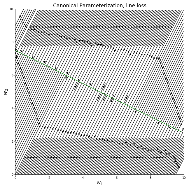
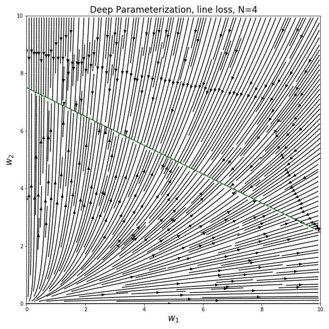
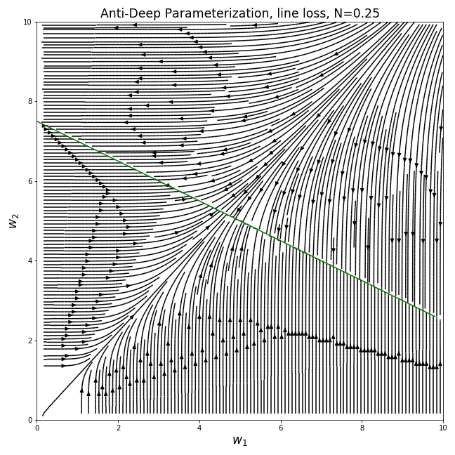
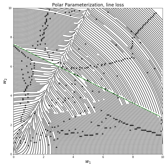
We can see that the different parameterizations converge to very different solutions for a given initialization, corresponding to the behaviors we noted for the previous loss. For example, the canonical parameterization over converges to the nearest point on the line from the initialization, while the deep parameterization clearly prefers sparser solutions…
In general, We see that when the function class we’re using to model our data is overly expressive, the parameterization has a very big effect on the solution we end up getting when we use gradient-based optimization. This is especially relevant for real-life nonlinear neural networks, even if describing the exact bias of their parameterization is currently out of our reach.
Conclusion
Hopefully, the plots and discussion in this post made it clear that gradient-based optimization behaves very differently under non-canonical parameterizations. In deep nonlinear networks it’s hard to even describe the canonical (linear) representation3, so any gradient-based optimization is bound to have these effects. Assuming we are able to carefully avoid the pitfalls caused by these effects (exploding and vanishing gradients for example), we’re left with particular biases towards specific types of solutions.
As we’ve hinted in this post, it seems that deep parameterizations initialized with small values relative to the solution (current deep learning best practice) bias the trajectory towards sparse solutions, and this could help explain why deep neural networks generalize so well even though they are supposedly too expressive to generalize.
This is an ongoing research direction that is currently restricted to relatively simple models, but the results we have so far suggest that studying the entire trajectory of networks during training is a strong way of understanding generalization.
Further Reading
If you found this post interesting, you’re more than welcome to look into our paper4, where we study the deep parameterization described in this post for small initializations and characterize the “incremental learning” dynamics that lead to sparse solutions. We then describe theoretically and empirically how this kind of dynamic leads many kinds of deep linear models towards sparse solutions.
Our research builds on many other works of the past few years that you may also be interested in:
The seminal paper that studied the dynamics of deep linear models was by Saxe et al5, where the authors derived gradient flow equations for deep linear networks under the squared loss and showed how different depths lead to different analytical solutions for the dynamics of the model. This work has since been extended to gradient descent6.
Another model that has been studied a lot in this context is matrix sensing, where both the input and model are parameterized as matices instead of vectors, and depth comes from linear matrix multiplication. The sparsity that is induced in these models is of low rank. The first work that seriously studied this model in this context was by Gunasekar et al7, followed by many other interesting works89.
While all of the above works deal with regression, there has also been very interesting work done on exponentially-tailed loss relevant for classification. For linear models over separable data, Soudry et al10 showed that gradient descent biases the solution towards the max-margin solution (minimum norm solution). However, deeply parameterized models behave differently for classification as well, as shown in Gunasekar et al11. Especially interesting, convolutional models tend towards sparsity in the frequency domain.
There’s also been some initial work on nonlinear models, either empirical12 or theoretical with restrictions on the data distribution1314.
Footnotes & References
-
This model and loss are very simple and useful for these demonstrations, but it is also related to real-life models and the squared loss. We can treat as a vector of parameters of a linear model, such that , and assume that there is indeed a that labeled our data. In that case, if our data comes from a standard Gaussian distribution, then the expected squared loss of over the data distribution is exactly this loss. This means that for linear models over Gaussian-like data distributions and the squared loss, the loss we’ll be discussing is a good approximation of the actual loss over our data. ↩
-
Note that the plots we show are only an approximation of the trajectories of gradient descent, since gradient descent uses a non-infinitesimal learning rate. These plots actually describe the trajectories of the optimization under an infinitesimal learning rate, otherwise called “gradient flow”. These dynamics are often an excellent approximation of the dynamics under small learning rates, and are a good way of getting a feel for the behavior of the optimization process. ↩
-
In the previous blog series we examined the canonical space of quadratic neural networks, and in general it is relatively simple to extend that discussion to polynomial networks that only have polynomial activations. However, once we have non-smooth activations that goes straight out of the window and we can’t describe the canonical space with a finite number of parametes. ↩
-
Gissin Daniel, Shalev-Shwartz Shai, Daniely Amit. The Implicit Bias of Depth: How Incremental Learning Drives Generalization. ICLR 2020. ↩
-
Andrew M Saxe, James L McClelland, and Surya Ganguli. Exact solutions to the nonlinear dynamics of learning in deep linear neural networks. arXiv preprint arXiv:1312.6120, 2013. ↩
-
Gauthier Gidel, Francis Bach, and Simon Lacoste-Julien. Implicit regularization of discrete gradient dynamics in linear neural networks. In Advances in Neural Information Processing Systems, pp. 3196–3206, 2019. ↩
-
Suriya Gunasekar, Blake E Woodworth, Srinadh Bhojanapalli, Behnam Neyshabur, and Nati Srebro. Implicit regularization in matrix factorization. In Advances in Neural Information Processing Systems, pp. 6151–6159, 2017. ↩
-
Sanjeev Arora, Nadav Cohen, Wei Hu, and Yuping Luo. Implicit regularization in deep matrix factorization. In Advances in Neural Information Processing Systems 32, pp. 7411–7422. Curran Associates, Inc., 2019. ↩
-
Blake Woodworth, Suriya Gunasekar, Jason Lee, Daniel Soudry, and Nathan Srebro. Kernel and deep regimes in overparametrized models. arXiv preprint arXiv:1906.05827, 2019. ↩
-
Daniel Soudry, Elad Hoffer, Mor Shpigel Nacson, Suriya Gunasekar, and Nathan Srebro. The implicit bias of gradient descent on separable data. The Journal of Machine Learning Research, 19 (1):2822–2878, 2018 ↩
-
Suriya Gunasekar, Jason D Lee, Daniel Soudry, and Nati Srebro. Implicit bias of gradient descent on linear convolutional networks. In Advances in Neural Information Processing Systems, pp. 9461–9471, 2018. ↩
-
Preetum Nakkiran, Gal Kaplun, Dimitris Kalimeris, Tristan Yang, Benjamin L Edelman, Fred Zhang, and Boaz Barak. Sgd on neural networks learns functions of increasing complexity. arXiv preprint arXiv:1905.11604, 2019. ↩
-
Remi Tachet des Combes, Mohammad Pezeshki, Samira Shabanian, Aaron Courville, and Yoshua Bengio. On the learning dynamics of deep neural networks. arXiv preprint arXiv:1809.06848, 2018. ↩
-
Francis Williams, Matthew Trager, Claudio Silva, Daniele Panozzo, Denis Zorin, and Joan Bruna. Gradient dynamics of shallow univariate relu networks. arXiv preprint arXiv:1906.07842, 2019. ↩