Over-Parameterization and Optimization I - A Gentle Start

Deep, over-parameterized networks have a crazy loss landscape and it’s hard to say why SGD works so well on them. Looking at a canonical parameter space may help.

Recently, there have been some interesting research directions for studying neural networks by looking at the connection between their parameterization and the function they represent. Understanding the connection between these two representations of neural networks can help us understand why SGD works well in optimizing these networks, and hopefully why SGD and over-parameterization seem to lead to strong generalization…

In this blog series I’ll review some of these concepts using toy examples, and develop some interesting ideas for how we can use this view to both develop new optimization algorithms, and explain the success of regular optimization methods for neural networks.

• Over-Parameterization
  • Parameteric and Canonical Spaces
  • Gradient Dynamics Between Spaces
  • A Variety of Parametric Gradients
  • Take-Aways From the Linear Example
• A More General View
  • The Loss Landscape
  • The Formation of “Ghost” Saddle Points
  • The Exploding and Vanishing Gradients Problem
  • Why the Canonical Gradient is so Canonical
• Exploring Parameterizations and Gradient Fields
  • Squared Parameterization
  • Inverse Parameterization
  • Polar Parameterization
  • Deep Linear Parameterization
• Further Reading
  • Deep Linear Networks
  • Non-Linear Networks
• Footnotes

Over-Parameterization

Neural networks are over-parameterized, meaning the same function can be represented by different sets of parameters of the same architecture. We can look at a simple example to demonstrate this - a two-layer linear neural network parameterized by the vector $v \in \mathbb{R}^{d}$ and the matrix $U \in \mathbb{R}^{d \times d}$, where out input is in $\mathbb{R}^{d}$:

$$f(x)=v^{T}Ux$$

Clearly, this is just a linear function, which means we only need $d$ dimensions in order to define it, but we have more than $d^{2}$. We have many ways of representing the same linear function with different parameters - if we permute the rows of $U$ and the entries of $v$ in the same way, the function will stay the same. If we multiply $U$ by a scalar and divide $v$ by that same scalar, the function will stay the same. These invariances of the model are relevant not only for linear networks, but for piece-wise linear as well (like ReLU networks).

You may ask - so what? As long as we are able to express a rich and relevant family of functions with our parameterized model, why should this over-parameterization matter to us?

We will now see that this over-parameterization leads to a very different optimization landscape for SGD.

Parameteric and Canonical Spaces

If we want to compare the two-layer linear network with the family of linear functions, we will need to define the two parameterizations and the way they are connected to each other. We already know what the parameteric space is - this is the over-parameterized model defined by $U$ and $v$. The canonical representation in our case will be the space of linear functions in $\mathbb{R}^{d} \rightarrow \mathbb{R}$, parameterized by $w \in \mathbb{R}^{d}$.

We call the canonical space “canonical”, because every set of parameters in it define a unique function, and every set of parameters in the parameteric space has a corresponding function in the canonical space. We are dealing with linear functions for now, so mapping from the parameteric space to the canonical is simply a matrix multiplication:

$$w(U,v)=U^{T}v$$

Note that we can’t map back from the canonical space to the parameteric, because the mapping isn’t bijective - a single $w$ has many possible parameterizations in the parameteric space… Also, note that while we are dealing with linear functions, the mapping between the two spaces is not linear in ${U,v}$.

Gradient Dynamics Between Spaces

Now that we’ve established these two spaces, both essentially representing the same functions, we can compare their gradient dynamics. Given an example $x \in \mathbb{R}^{d}$ and our convex loss function $\ell(f(x),y)$, we can write down the gradient of the loss with respect to the general parameters $\theta$ using the chain rule:

$$\frac{\partial \ell}{\partial \theta}=\frac{\partial \ell}{\partial f}\frac{\partial f}{\partial \theta}$$

We see that the parameters are only present in the derivative of the function $f$, so we can ignore the gradient of the loss and focus on the gradient of $f$ under the two different parameterizations. For the canonical space, the gradient is just the gradient of a linear function:

$$f(x) = w^{T}x$$ $$\frac{\partial f(x)}{\partial w} = x$$

For the parametric representation, we can use the chain rule to get the gradient (or calculate it directly):

$$f(x) = v^{T}Ux$$ $$\frac{\partial f(x)}{\partial v} = \frac{\partial f(x)}{\partial w}\frac{\partial w(U,v)}{\partial v} = Ux$$ $$\frac{\partial f(x)}{\partial U} = \frac{\partial f(x)}{\partial w}\frac{\partial w(U,v)}{\partial U} = vx^{T}$$

Now we start to see something interesting in the dynamics of the deep representation - while in the canonical space all functions have the same gradient with respect to $w$ (since the space is linear), in the deep representation the gradient depends on the parameterization. For example, given a fixed parameterization, if we increase the norm of all of the weights - the gradient will have a larger norm as well. This means that as training progresses and the norm of our weights increase (as they generally do), the gradients tend to grow as well (ignoring the gradient of the loss which usually becomes smaller).

We can see even more interesting phenomena when we look at the models after a small gradient step. Assuming we use an infinitesimal learning rate $\eta$, the model after a canonical gradient step will be:

$$\hat{f} = w - \eta \ell^{'}x$$

However, the model after a parameteric gradient step will be (ignoring second order terms of $\eta$):

$$\hat{f} = (v - \eta \ell^{'} v^{'})^{T}(U - \eta \ell^{'} U^{'}) = U^{T}v - \eta \ell^{'} (U^{T}Ux + v^{T}vx) = U^{T}v - \eta \ell^{'} (U^{T}Ux + ||v||^{2}x)$$

And look at this - we already know that the deep parameterization affects the norm of the gradient, but now we see that the deep parameterization also affects the direction of the gradient. The direction of the canonical gradient is along the axis defined by the input $x$, but the parameteric gradient is along the axis of the vector $U^{T}Ux + \left\lVert v\right\rVert^{2}x$.

A Variety of Parametric Gradients

Looking at the example above, it is interesting to explore how varied the direction and norm of the gradient can be, depending on the parameterization of the same function. There is a general transformation to the parameters of the deep model that we can look at that make the function remain the same - if we multiply $U$ by some invertible matrix $P$, and multiply $v$ by it’s inverse, we are left with the same function we started with:

$$(P^{-T}v)^{T}PU = v^{T}P^{-1}PU = v^{T}U$$

Now, this means that while a given function has a canonical gradient with a unique direction and norm, that same function in a two-layer parameterization can have many possible gradient directions and norms - each defined by an invertible $P$:

$$\nabla f = (U^{T}P^{T}PU + ||P^{-T}v||^{2}I)x$$

Basically, by choosing the right $P$ we can get a gradient to point anywhere we want in the positive halfspace of $x$ (since the matrix multiplying $x$ is PSD)!¹ If we can choose any two directions in a certain halfspace to be our gradient, it turns out that two different parameterizations of the same function could have negatively correlated gradients.

This is very interesting. The canonical space of functions we are working with is linear and we know a lot about how optimization works in it (namely, we can easily prove convergence for convex losses). However, once we over-parameterize a little we get completely different optimization dynamics which are much harder to deal with theoretically. These over-parameterized gradient dynamics depend on the parameterization at every time step, which means that if we want to guarantee convergence we have to pay attention to the entire trajectory of the optimization…

Take-Aways From the Linear Example

This 2-layer linear example is far from a deep convolutional ReLU network, but we can already see interesting phenomena in this example that exist in optimization of real networks.

The main thing we can gather from this example is the importance of balance netween the norms of the layers at initialization and during the optimization process. Looking at the parameteric gradient, $(U^{T}U + \left\lVert v\right\rVert^{2}I)x$, if either the norm of $v$ or the norm of $U$ is very large, then the gradient of the function will be huge even if the other’s norm is small. This means we need to initialize the parameters such that they have similar norms, like we do in practice. This issue arrises in real neural networks as the exploding/vanishing gradient problem…

Another interesting thing we can gather, is the possible importance of learning rate decay for deep models. For example, if the minimum of our loss function was some linear function with a very large $\ell_{2}$ norm, than a large learning rate could cause the dynamics to blow up when the parameters become large (since the gradient norm grows with the parameters). However, a small learning rate would take a very long time to converge. This suggests a new motivation for learning rate schedules that stems from the effects of the norm of our model on the gradient norm.

A More General View

In the next post I’ll be exploring non-linear neural networks, but before we get there we should take a step back and try to generalize what we just saw for deep linear networks.

We had two ways of looking at the same family of functions. The first was a canonical parameterization, where every function in our family had a unique parameterization and the function space was linear. The second was an over-parameterized representation, where every function in our family had many possible parameterizations. We also had a non-linear mapping from the parameteric space to the canonical one. Let’s define the canonical parameters as $\Theta \subset \mathbb{R}^{q}$ and the deep parmeterization’s parameters as $\mathcal{W} \subset \mathbb{R}^{p}$. The mapping between a deep parameterization $W$ and it’s corresponding $\theta$ can be written as $\psi:\mathcal{W} \rightarrow \Theta$.

So far we looked at how the gradients behave in the two spaces for the linear 2-layer example, but it should be interesting to see more generally how the loss landscape looks like between the two spaces.

The Loss Landscape

The first thing we care about in a loss landscape, is where are the critical points and are they well behaved?

For the canonical representation, if we assume that the functions in this representation are linear (like in our example and in future examples), then if the loss is convex we are very happy - there is a unique minimum to our function and we are guaranteed to reach it using SGD!²

As for the parametric representation, things aren’t necessarily as simple. As a quick example, we can look back at out linear example where $U=0$ and $v=0$. Looking at the gradients, this is a critial point of the loss landscape no matter what loss we have, and it generally isn’t a minimum (it’s a saddle point when the optimal function isn’t the zero function). So, if the canonical space has a unique critical point (the global minimum) but the parameteric space has more than one critial point - where did the additional critical points come from?

Well, we know how the two parameterizations are connected - they are connected by $\psi$. So, we can look like before at the gradients in the two spaces and ask when they are zero. Using the chain rule and the fact that $\psi(W)=\theta$:

$$\frac{\partial f}{\partial W} = \frac{\partial \psi(W)}{\partial W}\frac{\partial f}{\partial \psi(W)} = \frac{\partial \theta}{\partial W}\frac{\partial f}{\partial \theta}$$

For a given parameterization $W$, we see that the canonical and parameteric gradients are connected by a linear transformation define by the matrix $\frac{\partial \theta}{\partial W} \in \mathbb{R}^{p \times q}$. This immediately implies that if $\psi(W)$ maps to the unique global minimum of the canonical space, then it is also a critical point (a global minimum) of the parameteric space, since $\frac{\partial f}{\partial \theta} = 0$ and the relation between the gradients is linear. This is a nice sanity check…

However, the additional critical points come up in the situations where $\frac{\partial f}{\partial W} = 0$ and $\frac{\partial f}{\partial \psi(W)} \ne 0$. Since the connection between the gradients is through a matrix multiplication, this can happen only for $W$s for which the linear transformation between the two gradients is not full rank. In such a case, $\frac{\partial \theta}{\partial W}$ has a non-empty kernel and non-zero canonical gradients can be mapped to zero parameteric gradients, which means that we get a critical point where there is no such critical point in the canonical space.

The Formation of “Ghost” Saddle Points

So, For which $W$ is $\frac{\partial \theta}{\partial W}$ of partial rank?

To understand this, we need to more explicitly define $\frac{\partial \theta}{\partial W}$. Every column of this matrix defines how a single entry of $W$ changes every entry of $\theta$. If a set of these columns is linearly dependent, or equal to zero, the matrix can be of partial rank.

This happens for example when two row vectors of the same weight matrix in a neural network are identical/parallel (meaning two neurons are identical) - in such a case the two sets of columns will be linearly dependent. Another example can be “dead neurons” in ReLU networks - these neurons are always zero and so the outgoing weights from them don’t effect the actual model (and so their column is a zero vector).

In practice, when the neural network is large enough and the initialization is good, we don’t see this happening and the network is able to converge to a global minimum (with a loss of zero). Hui Jiang built on the above kind of reasoning in his paper to explain why highly expressive neural networks don’t get stuck in local minima even though there are so many in the loss landscape.

The Exploding and Vanishing Gradients Problem

Just like we explored the loss landscape using $\frac{\partial \theta}{\partial W}$, we can do the same sort of analysis to explain more generally why there are exploding and vanishing gradients.

Since $\frac{\partial \theta}{\partial W}$ depends on $W$, it is reasonable to believe (and it is the case in practice) that there are many $W$s for which the operator norm of $\frac{\partial \theta}{\partial W}$ is very large or very small. In such cases even though the canonical gradient is of a reasonable norm (assuming $x$ has bounded norm), $\frac{\partial \theta}{\partial W}$ could still increase/decrease the norm of the gradient considerably, causing the gradient to vanish or explode.

Why the Canonical Gradient is so Canonical

Finally, it is interesting to explore the interesting property we saw for the linear case, where for infinitesimal learning rates we always had a positive correlation between the parameteric gradient and the canonical one - is this a general property of over-parameterized models vs their linear canonical representation?

The answer is yes - if we have a linear canonical representation for our model and a differentiable function mapping a parameterization to that canonical representation, all gradients of the parameterizations of the same function will be positively correlated with the canonical gradient (while not necessarily positively correlated with each other).

Let’s prove it - we will denote our canonical parameterization as $\theta \in \mathbb{R}^{q}$ and the parameteric representation as $W \in \mathbb{R}^{p}$. We will denote the differentiable mapping from $W$ to $\theta$ as $\psi:\mathbb{R}^{p} \rightarrow \mathbb{R}^{q}$. Finally, we will denote the mapping of our input to the canonical linear space as $\phi: \mathcal{X} \rightarrow \mathbb{R}^{q}$.

We know that the function in the canonical space is linear, so we can easily write the function before and after an infinitesimal gradient step:

$$f_{c}(x) = \theta^{T}\phi(x)$$ $$\hat{f}_{c} = \theta - \eta \phi(x)$$

This means that the gradient of the canonical function in the canonical space is $\nabla f_{c} = \phi(x)$. We will now do the same process for the parametric gradient - we will calculate the change in $W$ and then map the new $\hat{W}$ to the canonical space. The gradient of $W$ can be calculated in the canonical space using our mapping $\psi$ and the chain rule:

$$f_{p}(x) = \psi(W)^{T} \phi(x)$$ $$\frac{\partial f}{\partial W} = \frac{\partial \psi}{\partial W} \frac{\partial f}{\partial \psi} = \frac{\partial \psi}{\partial W} \phi(x)$$

This means the new $W$ can be written in the following way:

$$\hat{W} = W - \eta \frac{\partial \psi}{\partial W} \phi(x)$$

We can now map that new parameterization to the canonical space and get our new canonical representation, after the gradient:

$$\hat{f}_{p} = \psi(W - \eta \frac{\partial \psi}{\partial W} \phi(x))$$

Since $\eta$ is infinitesimal, we can look at a first order approximation of $\psi$ around $W$ and neglect any higher order terms:

$$\hat{f}_{p} = \psi(W) + \frac{\partial \psi}{\partial W}^{T} (\hat{W} - W) = \psi(W) + \frac{\partial \psi}{\partial W}^{T} (-\eta \frac{\partial \psi}{\partial W} \phi(x)) = \psi(W) - \eta \frac{\partial \psi}{\partial W}^{T} \frac{\partial \psi}{\partial W} \phi(x)$$

We see the new function after a parametric gradient is indeed different from the one after a canonical gradient - in both cases we have a function that changes by adding a vector to the original function. In the canonical gradient step, that vector was $\nabla f_{c} = \phi(x)$, while in the parameteric step, that vector was $\nabla f_{p} = \frac{\partial \psi}{\partial W}^{T} \frac{\partial \psi}{\partial W} \phi(x)$.

Since $\frac{\partial \psi}{\partial W}$ in both cases is the Jacobian around the same $W$ (the initial $W$), $\frac{\partial \psi}{\partial W}^{T} \frac{\partial \psi}{\partial W}$ is PSD and so the two gradients are positively correlated.

Exploring Parameterizations and Gradient Fields

Before we move on to non-linear networks, it’s interesting to visualize just how much the parameterization we use can effect the gradient-based optimization of our model. Earlier, we saw that playing around with the parameterization of a deep linear network without changing the underlying function can drastically change the gradient of the function. Now, we will visualize this along with other possible parameterizations of linear functions!

We will visualize the dynamics by plotting the over-parameterized gradient on top of the canonical gradient. We will look at functions in $\mathbb{R}^{2}$ and for any original gradient value we will plot the one induced by the over-parameterization. We can look at the following example for regular canonical dynamics before we move on to more interesting dynamics:

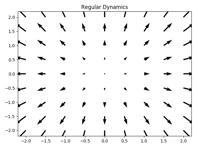
Every arrow’s starting point in the above plot is where the original gradient ended. The arrows are scaled down a bit to make things clear, so their direction and relative size are what we should look out for…

We see that in the regular dynamics, the canonical gradients remains the same - every arrow continues to point in the direction that it started in, and every arrow around a circle of the same radius has the same size. Let’s see how this changes with different parameterizations.

Squared Parameterization

Following a recent paper that studies the generalization effects of over-parameterization, we will look at a very simple linear function in $\mathbb{R}^{2}_{+}$. The canonical representation of such a function is simply $\theta \in \mathbb{R}^{2}_{+}$ - two positive numbers that are the coefficients of the inputs:

$$f_{\theta}(x) = \theta_{1}x_{1} + \theta_{2}x_{2}$$

However, we can use a different parameterization for our function, parameterized by $w \in \mathbb{R}^2$:

$$\theta_{i} = w_{i}^{2}$$ $$f_{w}(x) = w_{1}^{2}x_{1} + w_{2}^{2}x_{2}$$

This sort of parameterization is reminiscent of adding a layer to the linear neural network - the function remains the same but the gradient changes. As we saw, we can calculate how the gradient to $\theta_{i}$ should change when we are using this parameterization (and optimizing over $w$) by computing the PSD matrix $\frac{\partial \theta}{\partial w}^{T}\frac{\partial \theta}{\partial w}$ which multiplies the canonical gradient.

This matrix is diagonal since $\theta_{i}$ only depends on $w_{i}$, and we get the following diagonal entries:

$$\Big(\frac{\partial \theta}{\partial w}\Big)_{i,i} = 2w_{i} \rightarrow \Big(\frac{\partial \theta}{\partial w}^{T}\frac{\partial \theta}{\partial w}\Big)_{i,i} = 4w_{i}^{2}$$

This means that when w_{i} is large, we should expect the gradient to grow larger. On the other hand, if w_{i} is small we should expect the gradient to become smaller. This means that under this squared parameterization, the optimization is biased towards the features which are already deemed as important by the model. We can now look at the gradient field for different values of $w$:

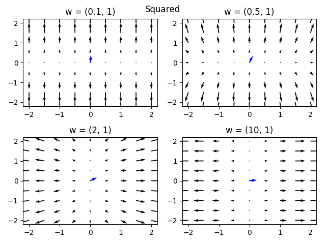
The blue arrow depicts the $w$ vector over the same axes. Indeed, we see that the gradients in this parmeterization are transformed so as to emphasize the gradients to parameters which are already large. In the extreme cases (top-left and bottom-right plots), we see that the function changes almost completely in the direction of the large weights, with little to no change to the small weights. This sort of parameterization induces sparsity - if we initialize the values of $w$ to be very small, then the weights more dominant in the optimization will get a head start and leave the other weights behind.

Inverse Parameterization

Just like we did for the squared parameterzation, we can use the following parameterization instead:

$$\theta_{i} = \frac{1}{w_{i}}$$ $$f_{w}(x) = \frac{1}{w_{1}}x_{1} + \frac{1}{w_{2}}x_{2}$$

We can now calculate the PSD matrix in the same way and get:

$$\Big(\frac{\partial \theta}{\partial w}^{T}\frac{\partial \theta}{\partial w}\Big)_{i,i} = \frac{1}{w_{i}^{4}}$$

We get the opposite of the squared parameterization - large values of $\theta$ are punished and their gradient is made smaller. We can see this in the gradient flow as well:

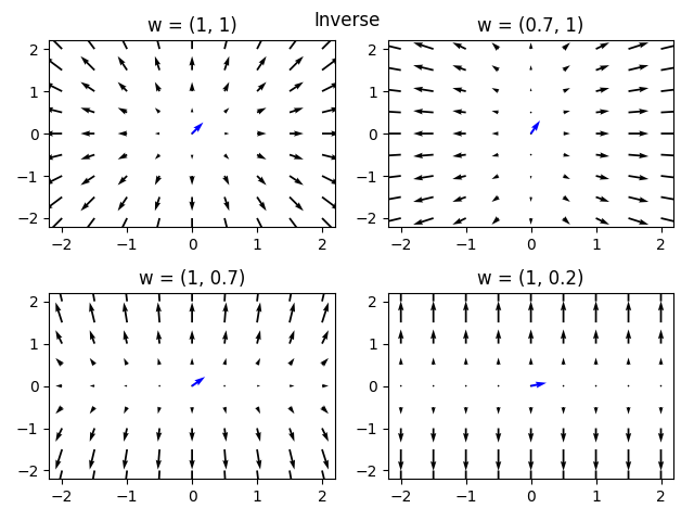
This parameterization has a strong bias towards weights that are relatively small in our model. It is reasonable to conjecture that this sort of parameterization is biased towards solutions with many small values for the weights, possibly minimizing the $\ell_{\infty}$ norm of the solution.

Polar Parameterization

We would be remiss not to look at the classic $\mathbb{R}^{2}$ parameterization - polar coordinates!

$$\theta_{1} = rcos(\varphi)$$ $$\theta_{2} = rsin(\varphi)$$ $$f_{polar}(x) = rcos(\varphi)x_{1} + rsin(\varphi)x_{2}$$

Like before, we can calculate the Jacobian matrix and visualize the gradient field for different parameterizations (changing $r$ this time):

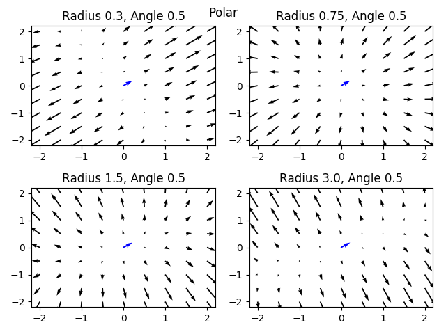
We see that this parameterization acts differently than the previous parameterizations - when $r=1$, we get the canonical gradient field. However, if $r$ is small we get a bias of the optimization towards the direction that the model is currently pointing to. If $r$ is large however, the optimization biases us towards the orthogonal direction to the current model.

I wouldn’t try to optimize my linear model under this parameterization, but it is pretty cool…

Deep Linear Parameterization

Finally, we can take a look at our original parameterization of a deep linear model, for the same function with different parameterizations determined by the invertible $P$ matrix. We will assume that $U=I$ and look at how different $P$ matrices change the optimization landscape:

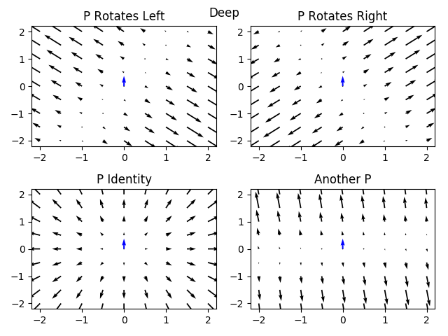
We see that we actually can completely change the optimization landscape by choosing different $P$ matrices, while the underlying function (the blue arrow) remains the same!

Further Reading

This sort of comparison between deep and canonical representations is used to both understand why neural networks are able to reach global minima of the loss landscape, and recently to start showing why they generalize well. In the next posts we’ll try exploring how we can develop optimization algorithms using this view.

Deep Linear Networks

A few papers from Sanjeev Arora and Nadav Cohen, along with other collaborators, address the dynamics of optimizing deep linear networks (deeper than our linear example).

The first paper studies depth and it’s effect on optimization. It shows that under certain assumptions on the weight initialization, depth acts as a preconditioning matrix at every gradient step (similar to the PSD matrix we saw in our small example). They also show that this kind of preconditioning cannot be attained by regularizing some type of norm of the canonical model - over-parameterization seems to be a different kind of animal than norm-based regularization.

In the second paper, the authors extend their results and show a convergence proof for deep linear networks under reasonable conditions on the random initialization.

In their recent, third paper, they move to studying generalization by showing that depth biases the optimization towards low rank solutions for a matrix completion/sensing task. There have been previous results showing that SGD creates this sort of bias and it is a strong belief today that SGD is a main factor in the generalization of neural networks. This work shows that not only does SGD bias us towards simple solutions, but that over-parameterization may also be a factor. As in the first paper, their results suggest that depth is a different animal than regularizing a norm (nuclear or otherwise), being more biased towards low rank than norm regularizations.

A nice paper by Ohad Shamir explores the optimization landscape of deep linear scalar networks, showing cases in which depth hurts optimization. In particular, Shamir shows that for certain conditions we need the number of gradient steps to convergence to be exponential in the depth of the network.

Finally, a recent paper by Nathan Srebro’s group analyzes an even simpler over-parameterization of the linear function - the squared parameterization discussed in the previous section. In their paper, the authors analyze the optimization at different initialization scales and show that in the limit of large initial weights, the model converges to the minimal $\ell_{2}$ solution, while in the limit of small initial weights, the model converges to the minimal $\ell_{1}$ solution, continuing the line of results showing that over-parameterization leads to clearly different implicit regularization. They also derive an analytic norm that is minimized for every scale of initialization, showing that the initialization-dependent solution moves from the minimal $\ell_{2}$ to the minimal $\ell_{1}$ continuously as we decrease the scale of initialization of the network.

Non-Linear Networks

This sort of analysis is very nice for linear networks where we can clearly define the canonical representation, which happens to be linear and behaves nicely. However, when we move to deep ReLU networks for example, we don’t even know how to properly describe the canonical representation, and it is incredibly high dimensional. Still, there are a couple of works that try to use the connection between the two spaces to explain why SGD works in the deep representation.

In Hui Jiang’s paper, the analysis of $\frac{\partial \theta}{\partial W}$ (refered to as the “disparity matrix”) is used to explore the loss landscape of general neural networks, assuming they are expressive enough. The canonical representation that is used is the Fourier representation of functions over the input space (which is also linear and nicely behaved). Assuming the family of neural networks $\epsilon$-convers that Fourier space (a strong assumption), this suggests that during optimization it would be very hard to have the diparity matrix not be of full rank, and therefore we shouldn’t be surprised that optimizing with SGD finds the global minimum.

Another paper by Julius Berner et al, analyzes shallow ReLU networks in order to start showing the connection between the parameteric space and canonical space (referred to as “realization space”) for an actual neural network. The main result shows “inverse stability” of the shallow neural network under certain, mild conditions on the weights. Informally, inverse stability is the property such that for a given parameterization $W$ and it’s corresponding canonical representation $\theta$, all canonical representations close to $\theta$ have a corresponding parametric representation close to $W$. Such a property suggests that optimizing in the parameteric space should behave like optimization in the canonical space. Another interesting thing in this paper, is that there is explicit discussion of the fact that while the canonical loss surface is convex (as we saw throughout this blog), shallow ReLU networks aren’t expressive enough to fill the entire canonical space. This means that the optimization objective in the canonical space is a convex loss function with a non-convex feasible set. We’ll see another, more digestible example of this in the next blog post.

---

---

Footnotes

1. The restriction to the halfspace of $x$ is true when $\eta$ is infinitesimal, otherwise we can’t neglect the $\eta^{2}$ term. In such a situation, which is what we see in actual SGD, the learning rate also plays a role in determining the direction of the gradient step. Also, large learning rates could even cause the gradient to step out of the halfspace of the canonical gradient, leading to a gradient step negatively correlated to the canonical one. ↩

2. Note that a linear canonical space is relevant for any kernel function simply by looking at the reproducing Hilbert space of the kernel. This means that we can mostly be safe in saying that there is some canonical representation which is linear. This space may be infinite-dimensional, but let’s not worry about that too much for now… ↩