Over-Parameterization and Optimization II - From Linear to Quadratic

If the canonical representation of the network has a nicer optimization landscape than the deep parameterization, could we use it to get better optimization algorithms for a non-linear neural network?

Last time, we looked at the connections between the regular parametrization of deep linear networks and their canonical parameterization as linear functions over $\mathbb{R}^{d}$. We saw that the deep parameterization introduced unnecessary critial points to the loss landscape, making it harder to guarantee convergence for gradient based optimization algorithms. There’s been some work explaining why this change to the loss landscape doesn’t hurt optimization, and maybe even why it can benefit generalization and optimization.

In this post however, we will try to see if we can optimize directly in the canonical space, which is linear and well-behaved. To make things interesting, we’ll look at a non-linear model for which we can do this kind of optimization - a “quadratic neural network”.

• The Quadratic Neural Network
  • Invariances in the Deep Representation
  • The Canonical Representation - Symmetric Matrices
• Optimizing the Quadratic Network
  • SGD in the Deep Representation
  • The Canonical Gradient
  • Theoretical Insights From the Canonical Representation
  • (Projected) SGD in the canonical representation
  • Toy Examples in the Low-Rank Domain
  • MNIST Experiments
• Footnotes

The Quadratic Neural Network

If you had to name the simplest possible non-linearity before ReLU because such a big deal, you would probably say that the squared activation was the simplest. It only requires multiplication of the input with itself, which is both very efficient computationally and means that the neural network is a realization of a polynomial function, which is something we know a lot about¹.

So, a step from linear networks towards deep ReLU networks could be a network with the squared activation. We will start by looking at a shallow network of that kind - our input will be $x \in \mathbb{R}^{d}$, which will be multiplied by a weight matrix $W \in \mathbb{R}^{r \times d}$. Then, every element will be squared, so our activation function is $\sigma(x)=x^{2}$. Finally, this hidden layer will be multiplied by a vector $\alpha \in \mathbb{R}^{r}$ to produce our prediction. Denoting the $i$‘th row of $W$ as $w_{i}$, we can write our function as following:

$$f(x) = \sum_{i=1}^{r} \alpha_{i}(w_{i}^{T}x)^{2}$$

A diagram of the network will look like this:

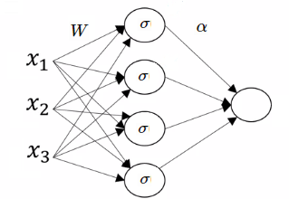
We immediately see that every set of parameters encodes a degree-2 polynomial over $\mathbb{R}^{d}$. As we’ll now see, this representation is over-parametrized in a very similar way to the linear example of our previous post.

Invariances in the Deep Representation

For deep linear networks, we saw that many different parameterizations actually encoded the same function. For example, we saw that multiplying and dividing two layers by the same scalar didn’t effect the function. We also saw that permuting the inputs and outputs of neurons in a corresponding way also did not change the function. These invariances return in our quadratic network, with slight changes.

First of all, the permutation invariance is the same - if we permute the rows of $W$ and the entries of $\alpha$ in the same order, it would simply be a different order of summation over the neurons. Since the order of summation doesn’t change the function, our parameterization is invariant to this kind of permutation.

Next, looking at a single neuron $\alpha (w^{T}x)^{2}$, if we multiply $w$ by a scalar $c$ while dividing $\alpha$ by $c^{2}$ - the neuron’s output doesn’t change:

$$\frac{1}{c^{2}} \alpha (c w^{T}x)^{2} = \frac{1}{c^{2}} c^{2} \alpha (w^{T}x)^{2} = \alpha (w^{T}x)^{2}$$

This means that we have an invariance to scalar multiplication of inputs and outputs of the same layer, when one scalar is the inverse square of the other.

These invariances suggest, like we saw last time, that there is some canonical parameterization for which every set of parameters encodes a unique function, and all functions from our family can be encoded. Luckily for us, it is easy to describe such a canonical space for the quadratic network.

The Canonical Representation - Symmetric Matrices

The quadratic neural network is a fancy name (and parameterization) of degree-2 polynomials. This means that we can use degree-2 polynomials over $\mathbb{R}^{d}$ as our canonical representation. This means our canonical parameterization has $\frac{d(d+1)}{2}$ free parameters - a coefficient for every pair of elements in $x$.

However, for convenience of notation and for a clearer geometric understanding, we will use an equivalent view of degree-2 polynomials - the view of such a polynomial as a quadratic form. Instead of viewing the polynomial as a linear function over the space of the products of pairs of elements in $x$, we can look at a polynomial as a symmetric matrix in $A \in \mathbb{R}^{d \times d}$². The polynomial function in this space can be described as both a quadratic form and a matrix inner product:

$$f(x) = x^{T}Ax = <A, xx^{T}> = Tr(A^{T}xx^{T})$$

Now we just need to map the network parameterization to this matrix parameterization, which can be done in the following way:

$$f(x) = \sum_{i=1}^{r} \alpha_{i}(w_{i}^{T}x)^{2} = \sum_{i=1}^{r} \alpha_{i}x^{T}w_{i}w_{i}^{T}x = \sum_{i=1}^{r} \alpha_{i}<w_{i}w_{i}^{T}, xx^{T}> = <\sum_{i=1}^{r} \alpha_{i}w_{i}w_{i}^{T}, xx^{T}>$$

So, our mapping from the parameterization of ${\alpha,W}$ to the parameterization of $A$ is:

$$A(\alpha,W)=\sum_{i=1}^{r} \alpha_{i}w_{i}w_{i}^{T}$$

Taking this matrix view instead of the regular degree-2 polynomial view gives us an additional geometric understanding of $r$, the number of hidden neurons in our network - it is the rank of the matrix! This leads us to the understanding that all degree-2 polynomials over $\mathbb{R}^{d}$ can be described using a quadratic neural network with $d$ hidden neurons.

Now that we have this geometrical understanding of our canonical space, we can move to seeing how this understanding can help us with optimizing our neural network - both in the full rank domain and the low rank domain.

Optimizing the Quadratic Network

Having described our model in two parameterizations, we can now choose in which one we will do our optimization. We can either optimize in the deep parameterization using SGD (as is usual for neural networks), or use SGD in polynomial/matrix space.

SGD in the Deep Representation

We can derive the gradients of the parameters either through backpropagation, or by explicitly calculating them from the matrix parameterization (by calculating $\frac{\partial A(W,\alpha)}{\partial \alpha}$ and $\frac{\partial A(W,\alpha)}{\partial W}$). The gradients turn out to be:

$$\frac{\partial f}{\partial \alpha_{i}} = (w_{i}^{T}x)^{2}$$ $$\frac{\partial f}{\partial w_{i}} = 2\alpha_{i}(w_{i}^{T}x)x$$

Like we saw for the linear example in the previous post, this parameterization creates “ghost” critial points which don’t exist in the canonical representation. These critical points are introduced by the parameterization, since the function isn’t linear in it’s parameters. For example, having $\alpha=0$ and $W=0$ makes the gradient of the function equal zero regardless of the loss (exactly like in the deep linear networks).

Another problem that comes up again, is the one introduced by the scalar multiplication invariance - an imbalance between $W$ and $\alpha$ can cause the gradients of the function to explode or vanish, and the gradients in general are highly dependent on the parameters.

This means that if we don’t initialize correctly when optimizing in this representation, we can run into problems.

The Canonical Gradient

Like we did for deep linear networks, we can look at the gradient of the canonical parameterization - that parameterization is linear³, so we should expect it to be independent of $A$. Indeed, the gradient of $f(x) = x^{T}Ax = <A,xx^{T}>$ is simply:

$$\frac{\partial f}{\partial A} = xx^{T}$$

This is great - we have a non-linear neural network that we can reason about using the same tools we used for the deep linear networks. We can now do the same thing we did for the linear case, and explore the effect of the deep parametrization on the gradients. Neglecting higher order terms of $\eta$, we can look at the deep model in the canonical representation, after a deep gradient step:

$$\hat{f} = \sum_{i=1}^{r} (\alpha_{i}-\frac{\partial f}{\partial \alpha_{i}})(w_{i} - \frac{\partial f}{\partial w_{i}})(w_{i} - \frac{\partial f}{\partial w_{i}})^{T}$$ $$= \sum_{i=1}^{r} \alpha_{i}w_{i}w_{i}^{T} - \eta \sum_{i=1}^{r} \big( (w_{i}^{T}x)^{2}w_{i}w_{i}^{T} + 2\alpha_{i}^{2}w_{i}^{T}x(w_{i}x^{T} + xw_{i}^{T}) \big)$$

And so, while the canonical gradient is simply $xx^{T}$, the deep gradient in it’s canonical form is:

$$\nabla_{deep} f = \sum_{i=1}^{r} \big( (w_{i}^{T}x)^{2}w_{i}w_{i}^{T} + 2\alpha_{i}^{2}w_{i}^{T}x(w_{i}x^{T} + xw_{i}^{T}) \big)$$

This expression is a bit less elegant than the linear network example, but it has the same kind of behavior as the linear case. We see that the gradient’s norm is dependent on the parameterization (and it’s balance between layers), as well as that the gradient’s direction is also dependent on the parameterization. We can see this by looking at the scalar invariance of the parametrization, where we can multiply $w$ by $c$ and divide $\alpha$ by $c^{2}$ (restricting ourselves to $r=1$ for simplicity):

$$\nabla_{deep} f = c^{4} (w^{T}x)^{2}ww^{T} + \frac{2}{c^{2}}\alpha^{2}w^{T}x(wx^{T} + xw^{T})$$

We see that as we play around with $c$, the gradient can be in any direction of the convex combination of $ww^{T}$ and $xw^{T}+wx^{T}$.

It is also easy to convince ourselves that the deep gradient, for an infinitesimal $\eta$, is always positively correlated with the canonical gradient⁴ (like the linear case, where the gradient was transformed using a PSD matrix). Seeing this behavior both in the linear and the quadratic case, we can understand how this should be the case for general linear canonical representations - the gradient will always be positively correlated with the canonical one, with it’s norm also being strongly dependent on the parameterization.

Theoretical Insights From the Canonical Representation

I should explain at this point that the quadratic model we’re talking about has been studied theoretically quite a bit. It has interested researchers because it is a non-linear neural network that is easier to probe theoretically than ReLU or sigmoid models. There are two papers that are most relevant to us when talking about SGD in the deep representation.

The first paper studies the loss landscape of the quadratic model by explicitly calculating it’s Jacobian and Hessian (not a fun experience). They show that if we have $2d$ hidden neurons and a fixed $\alpha$ vector, then all minima are global and all saddle points are strict. This means we should expect SGD to converge.

The second paper improves on the result and shows that under fixed $\alpha$ and with weight decay assumptions, it is enough to have $d$ hidden neurons for all minima to be global and all saddle points to be strict.

These results were hard work since they had to fight the artificially complex loss landscape caused by the over-parameterization. However if we look at the canonical representation of the model, this result is trivial and does not require any artificial assumptions like fixed weights or specific initialization. If we have $d$ hidden neurons, all of the symmetric matrices in $\mathbb{R}^{d \times d}$ are expressible by our model and so we have a convex optimization problem over a convex set, and SGD obviously converges with no further restrictions. This is a great win for the canonical representation view of the model, since it is much more elegant and clear description of the problem, allowing for minimal assumptions and a deeper understanding.

This view also highlights more clearly why the result is only valid for $d$ hidden neurons - the moment $r<d$, the symmetric matrices that can be expressed by our model are only those which are of rank $r$ or less. When $r<d$, this does not span all of the symmetric matrices and the problem in it’s canonical representation becomes a convex loss function over a non-convex feasible set. This means that our convex optimization knowledge is no longer enough, and we will need new ideas for reasoning about the low-rank domain.

While we think about new theoretical ideas for these kinds of optimization problems, we can still try to use the canonical representation to develop new optimization algorithms for our model, and that’s what we’ll do next.

(Projected) SGD in the canonical representation

Optimizing in the canonical space when $r = d$ is straightforward, since we simply do SGD until we converge (and we’re guaranteed to converge). However, when $r < d$, we are optimizing over a feasible set embedded in the linear space of symmetric matrices. We can still take gradient steps, but we will have to project our solution onto the feasiblt set (either at the end or after every gradient step).

So, we will need to know how to find the rank-$r$ matrix closest to a given symmetric matrix $A$. Every symmetric rank-$r$ matrix can be decomposed into the weighted sum of $r$ symmetric rank-$1$ matrices, which leads us to the following optimization problem for the projection:

$$\underset{W,\alpha}{argmin} || A - \sum_{i=1}^{r} \alpha_{i}w_{i}w_{i}^{T} ||^{2}_{F}$$

The solution to this optimization objective is to take the eigendecomposition of $A$ and setting $\alpha$ to be the $r$ largest eigenvalues (in absolute value) and $W$ to be the corresponding normalized eigenvectors. This also immediately gives us a way of obtaining the closest quadratic network with $r$ hidden neurons to a given symmetric matrix $A$.

We can now describe an optimization algorithm for the quadratic network that uses the canonical gradient step as opposed to the deep gradient. Given the model in it’s deep representation, we calculate it’s canonical representation as $A = \sum_{i=1}^{r} \alpha_{i}w_{i}w_{i}^{T}$ and take a gradient step of the form $A - \eta\ell^{'}xx^{T}$. We then perform an eigendecomposition of the matrix and set $W$ and $\alpha$ to be to top-$r$ spectrum of the matrix.

We can’t guarantee convergence for our projected algorithm when $r<d$ (the loss surface might have non-artificial local minima), but we can guarantee that we’ve solved the exploding/vanishing gradient problem. This algorithm is slower than regular SGD due to the eigendecomposition step, but if we use large mini-batches this difference disappears (at least theoretically, in a workd with no GPUs).

If you want to delve deeper into this optimization direction, you can take a look at this paper which develops a similar algorithm for the quadratic model, with a different projection step that tries to make the algorithm faster. They also give convergence guarantees under the assumption of Gaussian input and the squared loss.

Toy Examples in the Low-Rank Domain

The problem of optimizing a convex loss over a non-convex feasible set can be something hard to visualize. In these kinds of situations, it’s often advantageous to look at a toy example which should make thinks clearer and more visual. It’s also about time we saw a picture in this blog series…

If we want to visualize the low rank, non convex manifold embedded in canonical space, we will need to look at a low dimensional setting that allows it. Luckily, we can visualize the smallest low rank matrix manifold in $\mathbb{R}^{3}$. We will look at quadratic networks where $x \in \mathbb{R}^{2}$ that have one hidden neuron. This means our canonical representation is symmetric matrices in $\mathbb{R}^{2 \times 2}$, which can be parameterized using three parameters and visualized in $\mathbb{R}^{3}$ (this basically takes us back to the degree-2 polynomials coefficients parameterization). The rank-$1$ matrices of this form can be described as matrices of the form $\alpha ww^{T}$, with $\alpha \in \{\pm 1\}$ and $w \in \mathbb{R}^{2}$. This means that there are two real-valued parameters for our feasible set, which makes it a union of two-dimensional manifolds embedded in $\mathbb{R}^{3}$.

So, how does this union of manifolds embedded in the canonical space look like?

This plot shows the manifolds, where the axes correspond to the coefficients of the degree-2 polynomial $ax_{1}^{2} + bx_{2}^{2} + cx_{1}x_{2}$ (the rank-$1$ constraint gives us the equation $c=2ab$):

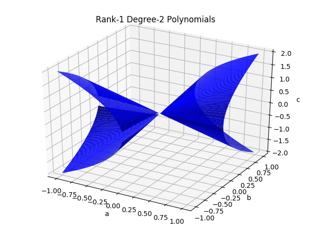
This is cool - we see that while the manifold is definitely non-convex as expected, it still has quite a bit of structure. The manifold consists of two cones that meet at the origin and go out in opposite directions. Optimizing in the deep parameterization makes every gradient step be restricted to this manifold, while optimizing in the canonical space means we take steps in the linear space in which the manifold is embedded, and then project back to the closest point on the manifold.

It is interesting to see in this visual example how the two algorithms perform and behave. They both make trajectories on this manifold, attempting to reach the global optimum, but their dynamics are quite different. Let’s look at the following experiment - we define a loss landscape over the symmetric matrices as being the squared loss between the model’s predictions and the optimal matrix’s prediction, where the input is Gaussian and the optimal matrix is rank-$1$, $\alpha_{*}w_{*}w_{*}^{T}$:

$$\ell(\alpha, w) = \underset{x \sim \mathcal{N}(0,I)}{\mathbb{E}}[(\alpha(w^{T}x)^{2} - \alpha_{*}(w_{*}^{T}x)^{2})^{2}]$$

We then minimize this loss, which is convex in the canonical spcae, using both optimization algorithms. We plot the trajectory of both algorithms throughout the optimization process, leads to the following trajectories:

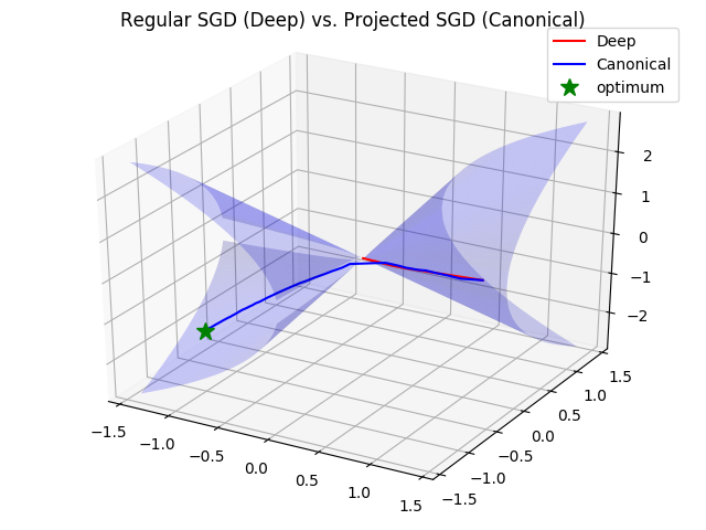
This is interesting - since the initial matrix and optimum matrix sit on separate manifolds, the optimization process had to go through the origin in order to reach the optimum. For the projected SGD algorithm this wasn’t a problem and the algorithm went through the origin (which isn’t a critical point) and reached the optimal matrix. However, the regular SGD has a critical point at the origin, and the closer we are to the origin the smaller the norm of the weights are, which cause the gradients to be small. The regular SGD experienced a vanishing gradient problem when it got close to the origin, causing the optimization to get stuck at the origin and not reach the second manifold…

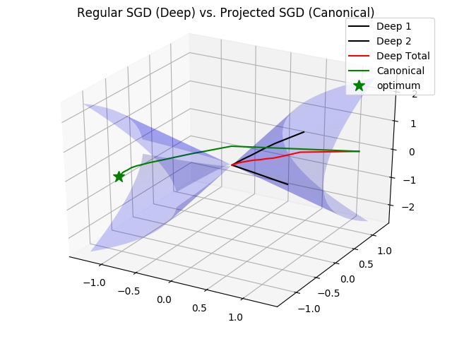
You may say that this problem is highly hand-crafted, and that it only happens when we restrict the matrix to be of rank-$1$. If it were full rank and able to span the entire canonical space, there should be no problem in optimizing the model with regular SGD because it wouldn’t be drawn into the origin and get stuck. The thing is, for SGD in the regular parameterization, every neuron’s output is restricted to the rank-$1$ manifold - the model is able to span the entire space only because it is a summation of these neuron outputs. For example, if we had two neurons on the same side of the manifold and the optimum was in the other halfspace, every neuron would have to separately cross the origin and they could both get stuck. We can see this example in the following plot, where the red line is the complete model trained with SGD, and the black lines are it’s two neurons (the optimum is a rank-$2$ matrix this time):

The last thing to note, which shows even more how the specific parameterization effect SGD, is that this pitfall of the dynamics can be avoided by careful scaling of $\alpha$, $W$ and the learning rate!

If we keep the same initialization but scale $W$ up and $\alpha$ down such that the model doesn’t change, the dynamics won’t get stuck at the origin because the gradients of $\alpha$ won’t vanish - $\frac{\partial f}{\partial \alpha_{i}} = (w_{i}^{T}x)^{2}$. However, if we adversarially choose the optimum to be such that $W$ has to change considerably, the optimization with SGD will still take a long time… You can see this in the next plot:

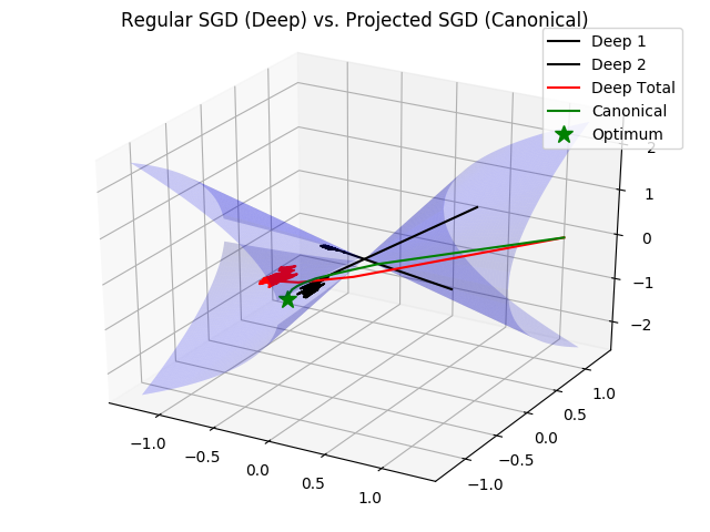
All of these experiments make us see that SGD in the deep representation can work, but it doesn’t work out of the box and requires careful understanding of the effects of the parameterization on the dynamics of optimization. This can make us want to go all in on the projection algorithm, but these sorts of pathological issue of SGD won’t necessarily replicate in higher dimensions. We can check this using a binary MNIST problem.

MNIST Experiments

To see if the projected SGD algorithm for the quadratic model is better than regular SGD for more realistic problems, we can try to solve the binary MNIST task (classifying 3s and 5s). In the following plot you can see learning curves of the two optimization algorithms, along with the corresponding Frobenius norm of each model in the canonical space. The rank for the model was chosen to be $r=10$, and the only difference aside from the optimization algorithms was the initialization, where the projected model was initialized with zeros since it is possible to do so (however, these results replicate for other initializations):

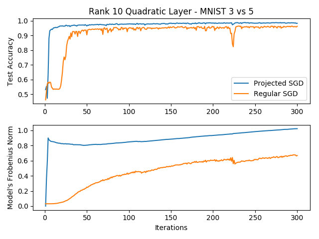
We can see several interesting things, the first of which is that the projection algorithm seems to perform much better than regular SGD in this low-rank regime. Not only is the accuracy much better, but the variance in the learning curve is smaller and more consistent. This result is reproduced under different initializations and learning rates, but I admit that I didn’t try playing around with the initialization like in the toy examples (I just used a standard Glorot initialization), and that could have improved the performance of SGD. We see that the complete breakdown of SGD we saw with the toy example does not happen with this high dimensional problem, but it is possible that the search space was restricted by the initializations of $\alpha$ that predetermined the manifold that every neuron will sit on, leading to a sub-optimal solution.

Another interesting thing to note is the model’s norm in the canonical space. The projected SGD has an initial large boost to the norm, caused by the large gradient of the loss function. It then changes very slowly, searching for the optimum. The regular SGD algorithm however, has a slowly increasing norm that is caused by the gradient being dampened by the initially small norm of the model. Once the model grows larger, the gradients grow as well, causing the optimization to be less stable.

However, we shouldn’t get too excited - if we use Adam as our optimizer for the deep representation, the optimization becomes more stable and the results are very similar to the projection algorithm. This is reasonable, since Adam can adjust the learning rate to be smaller when the model has a larger norm. Also, when the rank we use is larger ($r\approx50$), the advantage of the projected SGD algorithm over SGD dissappears completely. This can possibly be attributed to the fact that when $r$ is large, we have enough initial neurons in every manifold to express the optimal matrix…

You can get the code of this experiment here.

Still, this can make us hopeful about using this projected SGD algorithm in practice with these quadratic functions, and maybe even incorporate these models into a deep neural network. In order to do that and make our model and optimization algorithm practical, we need to generalize them such that they work with multiple outputs. This turns out not to be so straightforward, and we’ll tackle it in the next post.

---

---

Footnotes

1. It also has some advantages when we are dealing with private ML, since homomorphic encryptions work well with polynomials and multiplications, and not so well with functions such as the max function… ↩

2. Mapping the coefficients of $x_{i}$^{2} to the diagonal entries $A_{i,i}$ and mapping $\frac{1}{\sqrt{2}}x_{i}x_{j}$ to $A_{i,j}$ and $A_{j,i}$, we can see that the polynomial function is equivalent to $x^{T}Ax$. ↩

3. It isn’t a linear function of $x$, of course, but it is a linear function of the mapping $x \rightarrow xx^{T}$. When $x$ is mapped to the canonical Hilbert space, our function becomes a linear function. ↩

4. Taking the inner product with $xx^{T}$, we get: $\sum_{i=1}^{r} \big( (w_{i}^{T}x)^{2}x^{T}w_{i}w_{i}^{T}x + 2\alpha_{i}^{2}w_{i}^{T}x(x^{T}w_{i}x^{T}x + x^{T}xw_{i}^{T}x) \big) = \sum_{i=1}^{r} \big( (w_{i}^{T}x)^{4} + 4\alpha_{i}^{2}(w_{i}^{T}x)^{2}\left\lVert x\right\rVert^{2} \big) \ge 0$ ↩